


Background
Bayesian phylodynamics uses the shape of a phylogenetic tree to infer characteristics of the population represented in the phylogeny. Although widely applied to epidemiological datasets, the approach is yet to be used widely in macroevolution. In this case, skyline methods can be used to estimate parameters such as speciation, extinction and sampling rates over time, as well as the total number of lineages (usually species diversity). In this tutorial, we demonstrate how to apply piecewise exponential growth coalescent and fossilised-birth-death skyline models, which both estimate piecewise-constant evolutionary rates through time, to a dinosaur supertree. The models differ in the temporal direction in which they are applied, and the assumptions they make about how the phylogeny is sampled. We recommend reading the Skyline plots tutorial before attempting this one, as it covers a lot of the theory behind the models which we will not repeat here, except to highlight points which are relevant to macroevolutionary datasets.
Programs used in this Exercise
BEAST2 - Bayesian Evolutionary Analysis Sampling Trees 2
BEAST2 is a free software package for Bayesian evolutionary analysis of molecular sequences using MCMC and strictly oriented toward inference using rooted, time-measured phylogenetic trees (Bouckaert et al., 2014). This tutorial uses the BEAST v2.6.6.
BEAUti - Bayesian Evolutionary Analysis Utility
BEAUti2 is a graphical user interface tool for generating BEAST2 XML configuration files.
Both BEAST2 and BEAUti2 are Java programs, which means that the exact same code runs, and the interface will be the same, on all computing platforms. The screenshots used in this tutorial are taken on a Mac OS X computer; however, both programs will have the same layout and functionality on both Windows and Linux. BEAUti2 is provided as a part of the BEAST2 package so you do not need to install it separately.
Any programmer-friendly text editor
We will need to edit the XML files produced by BEAUti, for which we’ll need a text editor. It’s best to use one designed for programmers as these include nice features such as syntax highlighting, which makes the code more reader-friendly. Sublime Text is a good option which is available for MacOS, Windows and Linux.
Tracer
Tracer is used to summarise the posterior estimates of the various parameters sampled by the Markov Chain. This program can be used for visual inspection and to assess convergence. It helps to quickly view median estimates and 95% highest posterior density intervals of the parameters, and calculates the effective sample sizes (ESS) of parameters. It can also be used to investigate potential parameter correlations. We will be using Tracer v1.7.x.
R / RStudio
We will be using R to analyze the outputs of our analyses. RStudio provides a user-friendly graphical user interface to R that makes it easier to edit and run scripts. (It is not necessary to use RStudio for this tutorial.)
Practical: Skyline analyses for macroevolution
In this tutorial we will estimate diversification rates for dinosaurs using a previously published supertree. The evolutionary history of dinosaurs is somewhat controversial; although non-avian dinosaurs are well agreed to have become extinct as a result of an asteroid impact at the Cretaceous-Paleogene boundary, it has been fiercely debated whether the clade was already in decline prior to this event (e.g. (Brusatte et al., 2015; Benson, 2018)).
The aim of this tutorial is to:
- Learn how to set up a piecewise rate analysis using an existing (previously constructed) phylogeny;
- Develop skills in XML hacking;
- Highlight the differences between piecewise exponential growth coalescent and fossilised-birth-death skyline models.
If you have limited time, or only want to run part of the tutorial, we estimate that it should take:
- Set up piecewise exponential growth coalescent - 30-45 mins
- Set up fossilised-birth-death skyline - 30-45 mins (20-30 mins if you have already set up the other analysis)
- Analyse outputs - 20 mins
The data
We will be inferring our skyline parameters using a ready-made phylogeny containing 420 dinosaur species, published by (Lloyd et al., 2008). This phylogeny is a “supertree”, created using an informal method to collate several smaller dinosaur phylogenies into a larger one. Supertrees are typically cladograms, and must be timescaled using fossil data to estimate their branch lengths. The branch lengths we use here were inferred by (Sakamoto et al., 2016): they used fossil occurrences from the Paleobiology Database to define the temporal range of each species, used the midpoint of the temporal range for each tip date, and timescaled the phylogeny using the “equal” method, which distributes time evenly between the available branches.
Install BEAST2 packages
The piecewise exponential growth coalescent model is included in the BEAST2 core, but we will need to install the BDSKY package, which contains the fossilized-birth-death skyline model. We will also need the feast package, which will allow us to use a piecewise formulation of the model, and to integrate some more complex features into our analyses. Installation of packages is done using the package manager, which is integrated into BEAUti.
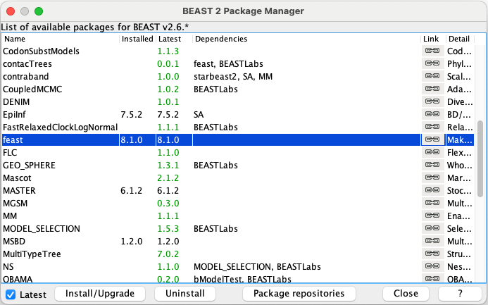
Open the BEAST2 Package Manager by navigating to File > Manage Packages.
Install the BDSKY and feast packages by selecting them and clicking the Install/Upgrade button one at a time.
After installing a package, it is on your computer, but BEAUti is unable to load the template files for the newly installed packages unless it is restarted.
Close the BEAST2 Package Manager and restart BEAUti to fully load the BDSKY and feast packages.
Setting up the Piecewise Exponential Growth Coalescent analysis
We will start with the simpler of the two models, the piecewise exponential growth coalescent. This model is somewhat similar in construction to the coalescent Bayesian skyline model used in the Skyline plots tutorial, but instead of assuming that the size of the population remains constant during our individual time intervals, we instead assume that they are experiencing exponential growth or decline at a constant rate throughout the interval, with instantaneous shifts in the growth rate between intervals. The advantage of using this model is that while the constant coalescent estimates constant effective population sizes within each time interval, we instead estimate diversification rates for each of the time intervals, which is what we would like to infer for our dinosaurs. Furthermore, whereas the coalescent Bayesian skyline model only allows interval boundaries to coincide with coalescent (or branching) times in the tree, we will use predefined time intervals, which will allow us to directly estimate diversification rates during our geological intervals of interest.
Many of the features we will need in our XML files are not currently implemented in BEAUti. However, for both models, we will start our analyses by creating XML files in BEAUti which will then serve as a template for us to alter by hand (“hack”) later.
Creating the Analysis Files with BEAUti
The first step in setting up an analysis in BEAUti is to upload an alignment. In our case, we do not have an alignment as we are using a ready-made phylogeny instead, but we will still need to upload an alignment in order to initialise our XML. We have a dummy .nexus file for this purpose, which we will replace later with code that reads in our phylogeny.
In the Partitions panel, import the nexus file with the empty alignment by navigating to File > Import Alignment in the menu and then finding the
empty.nexusfile on your computer, or drag and drop the file into the BEAUti window.
Most of the default tabs in BEAUti relate to inferring the phylogeny, which we will not be doing, so we can skip straight to the Priors tab. It’s worth remembering that a lot of the default parameters in BEAUti are set up for analyses very different to ours, so we need to check these thoroughly.
Select the Priors tab and choose Coalescent Exponential Population as the tree prior.
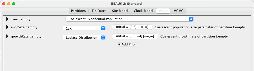
Here we see that the model has two parameters, ePopSize and growthRate. Our growthRate is simply our diversification rate. ePopSize refers to the effective population size at the start of the coalescent process. Because coalescent models consider time from the present backwards, this therefore refers to the size of the population at the end of our youngest time interval. The tips in our phylogeny are species, and so in this context, our effective population size can be considered to be a measure of the total species richness. Strictly speaking, it is an estimate of the number of species in the clade at the start of the coalescent process, under the assumption that these species act as a Wright-Fisher population (see Skyline plots tutorial). As this assumption is very likely violated, this value should be interpreted with caution in a macroevolutionary context.
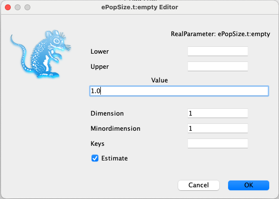
The default ePopSize prior is a 1/X distribution (or OneOnX), which is a reasonable choice when you have little knowledge about what the shape of your prior should be, placing reduced probability on higher values. However, it is not “proper”; a proper prior is one which is bounded, and therefore has an area under the curve equal to 1, which should ideally be the case when defining probability distributions. To meet this requirement, we will use a similarly shaped, but proper, lognormal distribution, with the default parameter values. We will also change the initialisation value (the value of the parameter in the first iteration of the chain) to 1.
Change the
ePopSizeprior to Log Normal, checking thatMis1.0andSis1.25.Click on the initial = button for
ePopSizeand change the initialisation value to 1.0.
The default growthRate prior is a Laplace distribution, but we will instead use a normal distribution, with diversification limits dictated by the magnitude of those estimated from living animals and plants (Henao Diaz et al., 2019). We will also set the initial growthRate estimate to 0.
Change the
growthRateprior to Normal, keeping themeanat0.0but changingsigmato0.5.Click on the initial = button for
growthRateand change the initialisation value to 0.0.
We will go into much more detail on the contents of this tab later, when setting up our birth-death model.
We can leave the rest of the tabs as they are and save the XML file. We want to shorten the chain length and decrease the sampling frequency so the analysis completes in a reasonable time and the output files stay small. Note that we won’t alter the treelog, because we won’t be using it, as our tree is fixed.
Navigate to the MCMC panel.
Change the Chain Length from 10’000’000 to 1’000’000.
Click on the arrow next to tracelog and change the File Name to
$(filebase).log, and make sure Log Every is set to 1’000.Leave all other settings at their default values and save the file as
dinosaur_coal.xml.Since we used
$(filebase).logas the name of the tracelog, the log file will be saved with the same name as our XML file, in this casedinosaur_coal.xml.
Amending the Analysis Files
We can now start “hacking” our XML template to ensure that it includes our desired features, including some that are not available in BEAUti.
Open
dinosaur_coal.xmlin your preferred text editor.
The first line sets out information about the format of the XML file and its contents, which we can ignore. The next section is labelled data, and contains our dummy alignment. We don’t need this section, so it can be commented out or simply deleted.
Remove the
datasection of the XML:<data id="empty" spec="Alignment" name="alignment"> <sequence id="seq_Tyrannosaurus_rex" spec="Sequence" taxon="Tyrannosaurus_rex" totalcount="4" value="N"/> </data>
In its place, we instead need to read in our phylogeny. We will do this by pasting in a new section, tree, which will use TreeFromNewickFile in the package feast to retrieve the phylogeny from our tree file, Lloyd.tree.
Where the
datasection was in the XML, paste in thetreesection:<tree id="tree" spec="feast.fileio.TreeFromNewickFile" fileName="Lloyd.tree" IsLabelledNewick="true" adjustTipHeights="false" />
The section after this contains a block of statements labelled map, which links the different distributions we might use (for example, for our priors) to the BEAST2 code which defines them. We will leave this alone, and move on to the largest and final block, run, which describes the analysis we want to carry out.
The first subsection within the run block is labelled state. This describes the objects inferred within the analysis (i.e. all of the model parameters we want to estimate). The first object described is the tree, based on our dummy alignment. As we are not inferring our tree, it can be removed from this section.
Remove the
treepart of thestatesubsection of the XML:<tree id="Tree.t:empty" spec="beast.evolution.tree.Tree" name="stateNode"> <taxonset id="TaxonSet.empty" spec="TaxonSet"> <alignment idref="empty"/> </taxonset> </tree>
After this we see descriptions of our two parameters, ePopSize and growthRate. Rather than one growth rate, we actually want to infer one for each of our time intervals of interest. To keep our analysis simple (in the hope of a timely convergence!), we are going to use four time bins, corresponding to the major geological intervals spanned by the phylogeny: the Triassic, Jurassic, Early Cretaceous and Late Cretaceous. We will therefore copy and paste the growthRate parameter three times, giving each a new name (id).
Convert the single
growthRateparameter into four with differentids:<state id="state" spec="State" storeEvery="5000"> <parameter id="ePopSize.t:empty" spec="parameter.RealParameter" name="stateNode">1.0</parameter> <parameter id="growthRate1" spec="parameter.RealParameter" name="stateNode">0.0</parameter> <parameter id="growthRate2" spec="parameter.RealParameter" name="stateNode">0.0</parameter> <parameter id="growthRate3" spec="parameter.RealParameter" name="stateNode">0.0</parameter> <parameter id="growthRate4" spec="parameter.RealParameter" name="stateNode">0.0</parameter> </state>
The next block, init, describes the initialisation processes, namely construction of the starting tree, which is a random tree simulated from an associated population model (here a constant-sized coalescent). Since we are reading in a previously constructed tree, our tree is already initialised, so we don’t need this block.
Remove the
initsubsection of the XML:<init id="RandomTree.t:empty" spec="beast.evolution.tree.RandomTree" estimate="false" initial="@Tree.t:empty" taxa="@empty"> <populationModel id="ConstantPopulation0.t:empty" spec="ConstantPopulation"> <parameter id="randomPopSize.t:empty" spec="parameter.RealParameter" name="popSize">1.0</parameter> </populationModel> </init>
The next block of the XML is arguably the most important: it defines the prior and posterior distributions of our analysis, including the model we are using. The model itself is described in the third nested distribution line, labelled CoalescentExponential. With the addition of line breaks to aid readability, it should currently look like this:
<distribution id="CoalescentExponential.t:empty" spec="Coalescent">
   <populationModel id="ExponentialGrowth.t:empty"
	spec="ExponentialGrowth"
	growthRate="@growthRate.t:empty"
	popSize="@ePopSize.t:empty"/>
   <treeIntervals id="TreeIntervals.t:empty" spec="TreeIntervals" tree="@Tree.t:empty"/>
</distribution>
The arguments determine the model to be used, and link the two parameters in the model, growthRate and popSize, to their definitions elsewhere in the XML. We can see that at present, the model uses a single growth rate for the full duration of the coalescent process. Instead of using this model, we are going to use a variation on it which is available in the package feast. This model is described as a CompoundPopulationModel, and allows multiple intervals to be defined over the course of our coalescent process, each of which can have their own population model. This will enable us to estimate a different diversification rate for each of our four time intervals of interest. The basic parameterisation of the model, as described on the feast Github page, is as follows:
<populationModel spec="CompoundPopulationModel">
    <populationModel spec="ConstantPopulation"> <popSize spec="RealParameter" value="5.0"/></populationModel>
    <populationModel spec="ConstantPopulation"> <popSize spec="RealParameter" value="10.0"/></populationModel>
    <populationModel spec="ConstantPopulation"> <popSize spec="RealParameter" value="2.0"/></populationModel>
    <changeTimes spec="RealParameter" value="1.0 3.0"/>
</populationModel>
We will be changing the ConstantPopulation specification to ExponentialGrowth, to match our desired model. We will also link the size of the population at the end of one interval as the starting population size in the next, using the makeContinuous="true" argument.
As well as defining models for three time intervals here, you can also see an object called changeTimes. Here we can provide a vector which describes when the boundaries between our time intervals should be, so it is easy for us to set these as our geological interval boundaries. The vector needs to provide the boundaries relative to the timescale of the phylogeny. We are assuming that the youngest tip lies at the Cretaceous-Paleogene boundary, so the times will need to describe the cumulative duration of these geological intervals relative to this boundary.
Replace the current
populationModelwith the following:<populationModel spec="feast.popmodels.CompoundPopulationModel" makeContinuous="true"> <populationModel spec="ExponentialGrowth" popSize="@ePopSize.t:empty" growthRate="@growthRate1"/> <populationModel spec="ExponentialGrowth" popSize="1.0" growthRate="@growthRate2"/> <populationModel spec="ExponentialGrowth" popSize="1.0" growthRate="@growthRate3"/> <populationModel spec="ExponentialGrowth" popSize="1.0" growthRate="@growthRate4"/> <changeTimes spec="parameter.RealParameter" value="32.55 77.05 133.35"/> </populationModel>
We also need to change the tree name in treeIntervals so that it links with the phylogeny we are reading in at the start of the XML.
Change
tree="@Tree.t:empty"totree="@tree"in thetreeIntervalsline.
As the fit of the model to the phylogeny is what we are interested in, we are going to rename this small block likelihood to ensure that this is what is recorded in our output logs.
Change
id="CoalescentExponential.t:empty"toid="likelihood".
The model block should now look like this:
<distribution id="likelihood" spec="Coalescent">
<populationModel spec="feast.popmodels.CompoundPopulationModel" makeContinuous="true">
          <populationModel spec="ExponentialGrowth" popSize="@ePopSize.t:empty" growthRate="@growthRate1"/>
          <populationModel spec="ExponentialGrowth" popSize="1.0" growthRate="@growthRate2"/>
          <populationModel spec="ExponentialGrowth" popSize="1.0" growthRate="@growthRate3"/>
          <populationModel spec="ExponentialGrowth" popSize="1.0" growthRate="@growthRate4"/>
          <changeTimes spec="parameter.RealParameter" value="32.55 77.05 133.35"/>
</populationModel>
<treeIntervals id="TreeIntervals.t:empty" spec="TreeIntervals" tree="@tree"/>
</distribution>
In the next few lines of our XML we can see that the shape of our prior distributions are defined. Our prior for ePopSize needs no further intervention beyond the settings we inputted into BEAUti. However, we only have a single GrowthRatePrior, but we now have four growthRate parameters, one for each of our time intervals. We need to copy and paste this prior three times, linking each prior to the diversification rate in one of those time intervals.
To tidy up, cut the
<distribution id="prior" spec="util.CompoundDistribution">line from above the model block and paste it below this block (immediately above theePopSizeprior).Copy and paste the
GrowthRatePriorblock three times, immediately below the first. Change the ` prior idandxnames to correspond to each of the fourgrowthRateparameters. Renumber theNormal idandparameter idnames so that each parameter has a differentid`.
The priors block should now look like this:
	   <distribution id="prior" spec="util.CompoundDistribution">
           <prior id="ePopSizePrior.t:empty" name="distribution" x="@ePopSize.t:empty">
               <LogNormal id="LogNormalDistributionModel.1" name="distr">
                   <parameter id="RealParameter.11" spec="parameter.RealParameter" estimate="false" name="M">1.0</parameter>
                   <parameter id="RealParameter.12" spec="parameter.RealParameter" estimate="false" lower="0.0" name="S" upper="5.0">1.25</parameter>
               </LogNormal>
           </prior>

           <prior id="GrowthRatePrior1" name="distribution" x="@growthRate1">
               <Normal id="Normal.1" name="distr">
                   <parameter id="RealParameter.1" spec="parameter.RealParameter" estimate="false" name="mean">0.0</parameter>
                   <parameter id="RealParameter.2" spec="parameter.RealParameter" estimate="false" name="sigma">0.5</parameter>
               </Normal>
           </prior>

           <prior id="GrowthRatePrior2" name="distribution" x="@growthRate2">
               <Normal id="Normal.2" name="distr">
                   <parameter id="RealParameter.3" spec="parameter.RealParameter" estimate="false" name="mean">0.0</parameter>
                   <parameter id="RealParameter.4" spec="parameter.RealParameter" estimate="false" name="sigma">0.5</parameter>
               </Normal>
           </prior>

           <prior id="GrowthRatePrior3" name="distribution" x="@growthRate3">
               <Normal id="Normal.3" name="distr">
                   <parameter id="RealParameter.5" spec="parameter.RealParameter" estimate="false" name="mean">0.0</parameter>
                   <parameter id="RealParameter.6" spec="parameter.RealParameter" estimate="false" name="sigma">0.5</parameter>
               </Normal>
           </prior>

           <prior id="GrowthRatePrior4" name="distribution" x="@growthRate4">
               <Normal id="Normal.4" name="distr">
                   <parameter id="RealParameter.7" spec="parameter.RealParameter" estimate="false" name="mean">0.0</parameter>
                   <parameter id="RealParameter.8" spec="parameter.RealParameter" estimate="false" name="sigma">0.5</parameter>
               </Normal>
           </prior>
       </distribution>
The last part of the distribution block is labelled the likelihood, and contains the treeLikelihood, which determines how well the inferred tree fits the sequences or morphological data. As we are using a fixed phylogeny and don’t have any other input data, we can remove this from our XML (we have already renamed our model the likelihood anyway).
Remove the
likelihoodblock containing thetreeLikelihood:<distribution id="likelihood" spec="util.CompoundDistribution" useThreads="true"> <distribution id="treeLikelihood.empty" spec="ThreadedTreeLikelihood" data="@empty" tree="@Tree.t:empty"> <siteModel id="SiteModel.s:empty" spec="SiteModel"> <parameter id="mutationRate.s:empty" spec="parameter.RealParameter" estimate="false" name="mutationRate">1.0</parameter> <parameter id="gammaShape.s:empty" spec="parameter.RealParameter" estimate="false" name="shape">1.0</parameter> <parameter id="proportionInvariant.s:empty" spec="parameter.RealParameter" estimate="false" lower="0.0" name="proportionInvariant" upper="1.0">0.0</parameter> <substModel id="JC69.s:empty" spec="JukesCantor"/> </siteModel> <branchRateModel id="StrictClock.c:empty" spec="beast.evolution.branchratemodel.StrictClockModel"> <parameter id="clockRate.c:empty" spec="parameter.RealParameter" estimate="false" name="clock.rate">1.0</parameter> </branchRateModel> </distribution> </distribution>
The penultimate block of the XML describes our operators. These define the moves that are used to propose new parameter values in the next iteration of the MCMC algorithm, so are fundamentally important to how our chain explores parameter space. Some are relevant to tree construction, so we can remove these.
Remove the tree operators:
<operator id="CoalescentExponentialTreeScaler.t:empty" spec="ScaleOperator" scaleFactor="0.5" tree="@Tree.t:empty" weight="3.0"/>
<operator id="CoalescentExponentialTreeRootScaler.t:empty" spec="ScaleOperator" rootOnly="true" scaleFactor="0.5" tree="@Tree.t:empty" weight="3.0"/>
<operator id="CoalescentExponentialUniformOperator.t:empty" spec="Uniform" tree="@Tree.t:empty" weight="30.0"/>
<operator id="CoalescentExponentialSubtreeSlide.t:empty" spec="SubtreeSlide" tree="@Tree.t:empty" weight="15.0"/>
<operator id="CoalescentExponentialNarrow.t:empty" spec="Exchange" tree="@Tree.t:empty" weight="15.0"/>
<operator id="CoalescentExponentialWide.t:empty" spec="Exchange" isNarrow="false" tree="@Tree.t:empty" weight="3.0"/>
<operator id="CoalescentExponentialWilsonBalding.t:empty" spec="WilsonBalding" tree="@Tree.t:empty" weight="3.0"/>
The next operator is a ScaleOperator which, when fired, scales the value of our ePopSize parameter. This is followed by a RealRandomWalkOperator, which alters our growthRate parameter via a random walk process. The first thing we will do is ensure that we have a RealRandomWalkOperator for each of our four growth rates.
Copy and paste the
RealRandomWalkOperatorthree times, and change theidandparameternames to our four separate growth rates, to create this:<operator id="GrowthRateRandomWalk1.t:empty" spec="RealRandomWalkOperator" parameter="@growthRate1" weight="3.0" windowSize="1.0"/> <operator id="GrowthRateRandomWalk2.t:empty" spec="RealRandomWalkOperator" parameter="@growthRate2" weight="3.0" windowSize="1.0"/> <operator id="GrowthRateRandomWalk3.t:empty" spec="RealRandomWalkOperator" parameter="@growthRate3" weight="3.0" windowSize="1.0"/> <operator id="GrowthRateRandomWalk4.t:empty" spec="RealRandomWalkOperator" parameter="@growthRate4" weight="3.0" windowSize="1.0"/>
One of the parameters in the RealRandomWalkOperator is the windowSize, which describes the permitted amplitude of parameter change. We will set this to 0.05 for each of our four rates.
Change the
windowSizeof each of thegrowthRateoperators to 0.05.
You can also see that each of our operators has a weight specified. This defines how often these operators fire relative to each other. All five of the weights have a value of 3.0, meaning that they are equally likely to fire. This is a reasonable set-up for our analysis so we will leave these values as they are.
And finally we reach the last block of the XML, which determines the logs outputted by our BEAST2 analysis. We can see a tracelog, which records our parameters to a log file, a screenlog, which provides settings on what is printed to the screen during the analysis, and a treelog, which records the trees sampled during our analysis. Our treelog would simply save identical versions of our input tree, so to save on file space we will remove it. We will also remove the OperatorSchedule - this can be useful for fine-tuning operators but we do not need it here.
Remove the
treelogandoperatorschedule:<logger id="treelog.t:empty" spec="Logger" fileName="$(tree).trees" logEvery="1000" mode="tree"> <log id="TreeWithMetaDataLogger.t:empty" spec="beast.evolution.tree.TreeWithMetaDataLogger" tree="@Tree.t:empty"/> </logger> <operatorschedule id="OperatorSchedule" spec="OperatorSchedule"/>
We also need to remove parameters from the tracelog and screenlog that no longer exist in our XML, and ensure that we are logging all four of our growthRate parameters.
Remove the
treeLikelihood,TreeHeight, andCoalescentExponentialparameters from thetracelog. Copy and paste<log idref="growthRate.t:empty"/>three times, changing theidreftogrowthRate1,growthRate2,growthRate3, andgrowthRate4.
With that, our XML is ready!
Save all changes to your XML file and close it.
We can now run the analysis in BEAST2. It’s important to have Lloyd.tree saved somewhere that BEAST2 can access it.
Download and save
Lloyd.treein the same folder as your BEAST2 program. Open the program and selectdinosaur_coal.xml(ordinosaur_coal_final.xmlif you’re using our ready-made version). Hit Run to start the analysis.OR
Download and save
Lloyd.treein the folder containing your XML file. Find the BEAST2 executable in BEAST_2.X.X (depending on your version) > bin. Right-click on the beast executable and select Create shortcut on Windows or Make alias on Mac. Cut and paste the created shortcut/alias into the folder containing your analysis files. If you open your terminal and navigate to the folder containing your files, you should now be able to run the analysis through the terminal usingbeast dinosaur_coal.xml(orbeast dinosaur_coal_final.xmlif you’re using our ready-made version).
The analysis should take about 5 minutes to run. In the meantime, you can start setting up the fossilised-birth-death analysis.
Setting up the Fossilised-Birth-Death Skyline analysis
As with the piecewise exponential growth coalescent model, many of the features we will need in our fossilised-birth-death XML file are not yet implemented in BEAUti, but we will start our analyses by creating template XML files in BEAUti.
Creating the Analysis Files with BEAUti
As before, we need to start by uploading our dummy .nexus file as an alignment.
In the Partitions panel, import the nexus file with the empty alignment by navigating to File > Import Alignment in the menu and then finding the
empty.nexusfile on your computer, or drag and drop the file into the BEAUti window.
Once again, we will skip straight to the Priors tab.
Select the Priors tab and choose Birth Death Skyline Contemporary BDSParam as the tree prior.
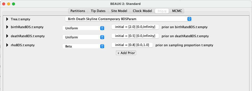
The “standard” contemporary birth-death skyline is parameterised using a reproductive number, a “become uninfectious” rate and a sampling proportion. However, here we are using the BDSParam model, which refers to the so-called “canonical” parameterisation, using a birth rate (here representing speciation), a death rate (here representing extinction) and an extant sampling probability (as defined in (Stadler, 2009)). As our phylogeny is of non-avian dinosaurs, for which we only have fossils and no extant (genetic) samples, we will later exchange the extant sampling probability, usually denoted using , for a fossil sampling rate, usually denoted using .
Choosing sensible priors for these parameters is not straightforward, so we will select priors which are relatively unrestrictive. For the birth and death rates, we will use exponential priors with a mean of 1.0; this places more weight on low rates, but still permits values which are towards the higher end of those estimated from living animals and plants (Henao Diaz et al., 2019). For the sampling rate, we will also choose an exponential prior, this time with a mean of 0.2.
On the initial = buttons you will see two sets of square brackets. The first indicates what the starting value for that parameter will be; we always need to check our initialisation values to ensure that they sit within our prior distributions. The second contains two values which denote the limits of the range of values that our parameters are permitted to take, which are also important to consider carefully. The prior distribution influences the probability of certain parameter values being sampled in the MCMC chain, but values across the entire prior range, even very improbable values, can still be sampled. This is especially true if there is a strong signal for such parameter values in the data (high likelihood). If we have a strong reason to believe such parameter values are unrealistic, we can (and should) use parameter limits to exclude them. Setting finite upper and lower bounds in effect changes the prior to be the specified prior distribution multiplied by a uniform distribution on this range. Note that when no prior distribution is explicitly specified in BEAST2, the prior is then just a uniform prior across the parameter range (all parameters therefore have priors). Our parameters are all rates, expressed per branch per million years, so the full set of values they can take ranges between 0 and infinity. (For now, the rho parameter is defined between 0 and 1 because it is a sampling probability; later we will change this to a sampling rate, defined between 0 and infinity.)
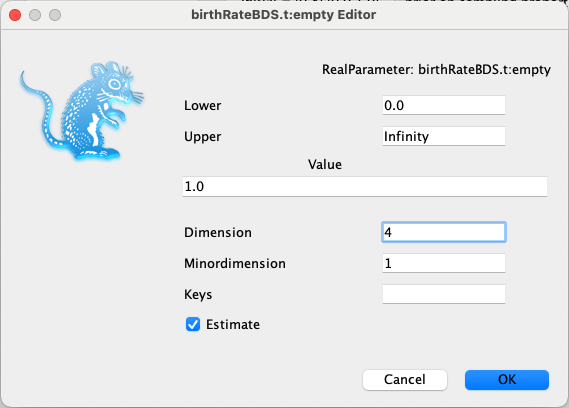
This is also the point where we express how many sections (here called dimensions) we want in our piecewise constant rates. Our rates will be assumed to be constant within these sections, but will be permitted to change at the break points between them. Similar to the exponential coalescent model, we are going to give our rates four dimensions, corresponding to the Triassic, Jurassic, Early Cretaceous and Late Cretaceous.
Change the birth rate prior from a uniform distribution to an exponential. Using the drop-down arrow on the left, check that the mean is set to 1.0. Click on the initial = button and change the initialisation value to 1.0. Check that the lower value is 0.0 and the upper value is
Infinity. Change the Dimension to 4. Repeat these four steps for the death rate prior.Change the rho (sampling) prior from a uniform distribution to an exponential. Using the drop-down arrow on the left, change the mean value to 0.2. Click on the initial = button and change the initialisation value to 0.5. Check that the lower value is 0.0, and change the upper value to
Infinity. Change the Dimension to 4.
We can leave the rest of the tabs as they are and save the XML file. We will again shorten the chain length and decrease the sampling frequency of our analysis, so the analysis completes in a reasonable time and the output files stay small.
Navigate to the MCMC panel.
Change the Chain Length from 10’000’000 to 5’000’000.
Click on the arrow next to tracelog and change the File Name to
$(filebase).log, and make sure Log Every is set to 1’000.Leave all other settings at their default values and save the file as
dinosaur_BDSKY.xml.
Amending the Analysis Files
It is now time to “hack” our XML template, to remove the content we don’t need and add some additional features. The first few steps are the same as for our exponential coalescent XML.
Open
dinosaur_BDSKY.xmlin your preferred text editor.Remove the
datasection of the XML:<data id="empty" spec="Alignment" name="alignment"> <sequence id="seq_Tyrannosaurus_rex" spec="Sequence" taxon="Tyrannosaurus_rex" totalcount="4" value="N"/> </data>Where the
datasection was in the XML, paste in thetreesection:<tree id="tree" spec="feast.fileio.TreeFromNewickFile" fileName="Lloyd.tree" IsLabelledNewick="true" adjustTipHeights="false" />Remove the
treepart of thestatesubsection of the XML:<tree id="Tree.t:empty" spec="beast.evolution.tree.Tree" name="stateNode"> <taxonset id="TaxonSet.empty" spec="TaxonSet"> <alignment idref="empty"/> </taxonset> </tree>
Following this we see a description of our three inferred rates: birth, death and sampling. These lines include a lot of information, much of which we specified earlier via the Priors tab in BEAUti. As previously mentioned, our sampling parameter is currently set up as the extant sampling probability, rho, which we want to exchange for a fossil sampling rate, sampling. For the sake of readability, we will change the id (name) of our sampling parameter here from rhoBDS to samplingBDS. Here, this is simply a label and does not change what the parameter does, but it is how the parameter is referenced in other parts of the XML, where its name will also need to be changed.
Replace all instances of
rhoin the XML withsampling. There should be eight. This is most easily (and reliably) done using theFind & Replacefunctionality.
To our three rates we will also add a fourth parameter, origin. This denotes the time at which the evolutionary process started, in our case the origin of the dinosaur clade. Here we need to set the limits of our origin time and its initial value. BEAST2 assumes that time runs from the present backwards (as is the case in our Exponential Coalescent model), so we will set our origin’s lower limit to 0 (the age of the youngest tip), and to be maximally conservative, its upper limit to Infinity. We will set the starting value to 200 (200 million years before the youngest tip), which corresponds to an age of approximately 200 + 66 = 266Ma (if our youngest tip lies at the Cretaceous-Paleogene boundary, when non-avian dinosaurs are thought to have become extinct). This would place the origin of dinosaurs during the middle Permian, which is perhaps a little earlier than most palaeontologists would speculate (Early to Middle Triassic, e.g. (Brusatte et al., 2010; Langer et al., 2010)), but is certainly adequate for our first iteration.
Paste in the
originline to the end of theparameterblock:<parameter id="origin.t:empty" spec="parameter.RealParameter" lower="0.0" name="stateNode" upper="Infinity">200.0</parameter>The
stateblock should now look like this:<state id="state" spec="State" storeEvery="5000"> <parameter id="birthRateBDS.t:empty" spec="parameter.RealParameter" dimension="4" lower="0.0" name="stateNode" upper="Infinity">1.0</parameter> <parameter id="deathRateBDS.t:empty" spec="parameter.RealParameter" dimension="4" lower="0.0" name="stateNode" upper="Infinity">1.0</parameter> <parameter id="samplingBDS.t:empty" spec="parameter.RealParameter" dimension="4" lower="0.0" name="stateNode" upper="Infinity">0.5</parameter> <parameter id="origin.t:empty" spec="parameter.RealParameter" lower="0.0" name="stateNode" upper="Infinity">200</parameter> </state>
Note that each of our rate parameters have 4 dimensions but that we do not specify this value for our origin; while our piecewise constant rates will have four values in each iteration (one for each time interval), only a single origin value is needed, and we therefore do not need to specify its number of dimensions (as 1).
As before, the init block is not needed for this analysis.
Remove the
initsubsection of the XML:<init id="RandomTree.t:empty" spec="beast.evolution.tree.RandomTree" estimate="false" initial="@Tree.t:empty" taxa="@empty"> <populationModel id="ConstantPopulation0.t:empty" spec="ConstantPopulation"> <parameter id="randomPopSize.t:empty" spec="parameter.RealParameter" name="popSize">1.0</parameter> </populationModel> </init>
The next block describes the model, which is labelled BirthDeathSkyContemporaryBDSParam. With the addition of line breaks to aid readability, it should look like this:
	<distribution id="BirthDeathSkyContemporaryBDSParam.t:empty"
                          spec="beast.evolution.speciation.BirthDeathSkylineModel"
                          birthRate="@birthRateBDS.t:empty"
                          conditionOnRoot="true"
                          contemp="true"
                          deathRate="@deathRateBDS.t:empty"
                          sampling="@samplingBDS.t:empty"
                          tree="@Tree.t:empty">
Although perhaps initially intimidating, we will walk through the various arguments here and what they mean. The model will also require some tweaking to fit our intended usage.
The first thing to note is that we’re linking the parameters we defined earlier into the model. For example, birthRate="@birthRateBDS.t:empty" is simply telling the model the name we have given to our birth rate parameter. This is also true for deathRate. If you successfully changed all of the rho references to sampling earlier, you should also see that sampling="@samplingBDS.t:empty". The name of the argument in the model is actually samplingRate, so we will correct that now.
Change
sampling="@samplingBDS.t:empty"tosamplingRate="@samplingBDS.t:empty".
We also need to link the origin parameter (which we defined earlier) into the model.
Somewhere within the model line, add
origin="@origin.t:empty".
The next argument to note is conditionOnRoot="true". Conditioning refers to the process of tuning the model settings to align with our prior knowledge about the specific evolutionary system we are investigating. The different directions of time between coalescent and birth-death models means that this process is fundamentally different between the two. Our coalescent model is conditioned on fitting the input data, our sampled phylogeny. However, in birth-death models, our sampled phylogeny is instead an output of the process, and so we need to provide additional information about how the model should work. In BDSKY, there are two main ways to condition our model: determining when the evolutionary process is considered to have started, and whether (or how) the process has been sampled.
The first of these settings is determined using the conditionOnRoot parameter. When conditionOnRoot="true", we are telling BDSKY to commence our evolutionary process at the root of the tree; in macroevolution, this corresponds to our first speciation event, when the most recent common ancestor (MRCA) of our clade first diverged into two daughter species. Using this setting allows us to place a prior on the timing of the root of the tree. When conditionOnRoot="false", we are telling BDSKY to instead commence our evolutionary process at the origin; this is when the first branch in the tree initially appeared. In doing so, we are including this initial branch within our clade. Using this setting allows us to place a prior on the timing of the origin, rather than the root. As we discussed before, we intend to place a prior on the origin, and consider this initial branch to be our first dinosaur, meaning that it should be included in our evolutionary process. We therefore want to set conditionOnRoot="false". This is the default setting, and so we can simply remove this parameter specification from our XML.
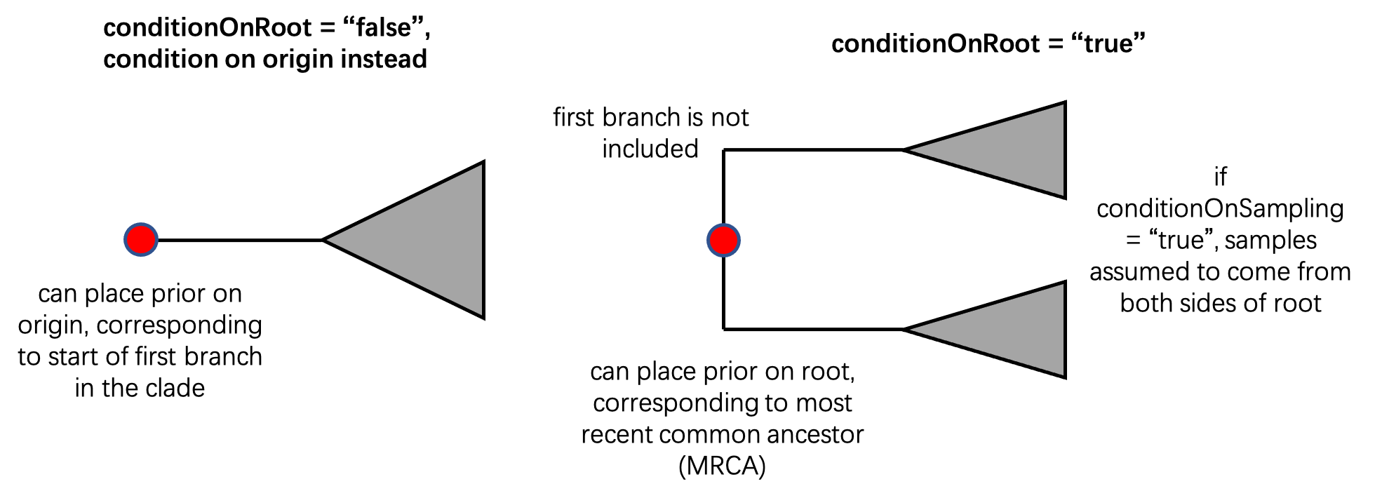
The second way to condition our BDSKY model is to ensure that the model produces at least one sample (is observable). Depending on the relevant type of sampling, we can either use conditionOnRhoSampling or conditionOnSurvival: the former assumes at least one extant sample, while the latter assumes at least one sample of either type (an extant sample or an observed fossil). It’s worth noting that when conditionOnRoot="true", the model assumes that our samples are drawn from both sides of the root, and therefore that the MRCA in the sampled tree corresponds to the MRCA in the “true” tree. As our phylogeny of non-avian dinosaurs only includes extinct species, we will set conditionOnRhoSampling="false" and conditionOnSurvival="true".
Change
conditionOnRoot="true"toconditionOnSurvival="true" conditionOnRhoSampling="false".
After this is the argument contemp="true". When true, this means that all samples were collected at the same time (assumed to be the present, i.e. contemporaneous) and is the default setting for the Birth Death Skyline Contemporary BDSParam parameterization in BEAUti. Since our dataset is not homochronous, but we instead have heterochronous samples (in our case fossils that were deposited at different times), and no extant samples, we should set contemp="false". However, the default for the fossilized-birth-death skyline is contemp="false", so we can simply delete the line.
For our fossil sampling rate, we instead need to specify a different parameter, the removalProbability. When applying birth-death models to epidemiological datasets, sampling events are often assumed to be associated with removal; once patients have been sampled and their pathogens sequenced (which adds them to the phylogeny), it is assumed that they are removed from the infectious population, either through isolation or successful treatment and that they cannot subsequently infect anyone else. For our dataset, this assumption would prevent multiple fossils from existing for any single species, and mean that species for which fossils have been found could not be direct ancestors of other species in the phylogeny. In effect, this would be equivalent to assuming that fossils are only deposited at the time of extinction. We can set the removalProbability to relax this assumption, and allow so-called “sampled ancestors”. While the relevance of this assumption to supertrees is debatable, it is logical to set removalProbability to 0 for fossil phylogenies, since the probability is vanishingly small that any species went extinct exactly at the time a fossil was deposited (see (Gavryushkina et al., 2014)).
Change
contemp="true"toremovalProbability="0.0".
The last argument currently in the model line links the tree into the model. We need to update the name of the tree object to correspond to our fixed phylogeny, which we read in at the start of the XML.
Change
tree="@Tree.t:empty"totree="@tree".
The model is almost ready, but we want to add one last set of arguments to it. Our rates are piecewise constant, and we have already specified in the state block how many dimensions (constant intervals) each of our rates will have. By default, the break points in our rates are evenly spaced between the origin and the youngest tip, meaning that all of the intervals are the same length. However, we can add arguments to our model specifying when we would like our break points to be. For us, it makes sense to place these break points at the boundaries of geological intervals, so that we estimate a rate for each interval. As mentioned before, we are going to align our break points to the boundaries between the Triassic, Jurassic, Early Cretaceous and Late Cretaceous. To do this, we need to supply vectors of these times relative to the phylogeny. We are assuming that the youngest tip, at which t=0, lies at the Cretaceous-Paleogene boundary, so the vectors describe the cumulative duration of these geological intervals relative to this boundary. We need to specify a separate vector for each of our rates.
Add to the end of the model line:
birthRateChangeTimes="0 32.55 77.05 133.35"
deathRateChangeTimes="0 32.55 77.05 133.35"
samplingRateChangeTimes="0 32.55 77.05 133.35"
Beneath our model, you will see a line which sets the samplingRate to 0. This refers to fossil sampling, which we have now introduced into our model, so this line needs to be removed.
In its place, we instead need to add an instruction to the XML about the direction of time. The birth-death skyline model implemented in BEAST2 assumes that time runs forwards, from the origin to the present. That means that by default it assumes the break point times are measured forward-in-time from the origin. However, we specified our break point times as offsets backward-in-time from the youngest tip. We did this because we know the age of the youngest tip exactly, but we don’t know the age of the origin (we are estimating it instead). To switch the time direction for the break point times, we use the reverseTimeArrays parameter. Here, we are telling the model to use the opposite direction of time to the default in five dimensions: in order, this refers to our three rate parameters (birth, death and sampling) plus rho and the removalProbability (which we do not need but will specify anyway).
Remove the line fixing
samplingRateto 0:<parameter id="samplingRateBDS.t:empty" spec="parameter.RealParameter" name="samplingRate">0.0</parameter>Replace it with an instruction to
reverseTimeArrays:<reverseTimeArrays id="BooleanParameter.0" spec="parameter.BooleanParameter" dimension="5">true true true true true</reverseTimeArrays>
And with that our model is complete! In summary, the model should now read (with arguments in any order):
	<distribution id="BirthDeathSkyContemporaryBDSParam.t:empty"
                          spec="beast.evolution.speciation.BirthDeathSkylineModel"
			  origin="@origin.t:empty"
                          birthRate="@birthRateBDS.t:empty"
			  deathRate="@deathRateBDS.t:empty"
                          samplingRate="@samplingBDS.t:empty"
                          conditionOnSurvival="true"
			  conditionOnRhoSampling="false"
                          removalProbability="0.0"
                          tree="@tree"
			  birthRateChangeTimes="0 32.55 77.05 133.35"
			  deathRateChangeTimes="0 32.55 77.05 133.35"
			  samplingRateChangeTimes="0 32.55 77.05 133.35">
	<reverseTimeArrays id="BooleanParameter.0" spec="parameter.BooleanParameter" dimension="5">true true true true true</reverseTimeArrays>
	</distribution>
The next part of our XML specifies the shape of our prior distributions. As long as you changed all of the rho references to sampling previously, we don’t need to modify the priors we already have any further; we provided all of the necessary information in BEAUti. We do, however, need to add a prior on our origin. You may remember that when specifying the parameter, we set our starting value to 200 (corresponding to 266Ma). To keep things simple, we will set the origin prior to a uniform distribution between 0 and 200.
Add an
originprior to thepriorsblock:<prior id="originPrior" name="distribution" x="@origin.t:empty"> <Uniform name="distr" upper="200"/> </prior>
As before, the last part of the distribution block is labelled the likelihood, and contains the treeLikelihood, which we don’t need because we are using a fixed phylogeny. What we consider the likelihood in our analysis is instead how well the model parameters fit our phylogeny, so this time we will cut and paste our fossilized-birth-death model into this part of the XML.
Remove the
treeLikelihoodblock from thelikelihoodpart of the XML:<distribution id="likelihood" spec="util.CompoundDistribution" useThreads="true"> <distribution id="treeLikelihood.empty" spec="ThreadedTreeLikelihood" data="@empty" tree="@Tree.t:empty"> <siteModel id="SiteModel.s:empty" spec="SiteModel"> <parameter id="mutationRate.s:empty" spec="parameter.RealParameter" estimate="false" name="mutationRate">1.0</parameter> <parameter id="gammaShape.s:empty" spec="parameter.RealParameter" estimate="false" name="shape">1.0</parameter> <parameter id="proportionInvariant.s:empty" spec="parameter.RealParameter" estimate="false" lower="0.0" name="proportionInvariant" upper="1.0">0.0</parameter> <substModel id="JC69.s:empty" spec="JukesCantor"/> </siteModel> <branchRateModel id="StrictClock.c:empty" spec="beast.evolution.branchratemodel.StrictClockModel"> <parameter id="clockRate.c:empty" spec="parameter.RealParameter" estimate="false" name="clock.rate">1.0</parameter> </branchRateModel> </distribution> </distribution>Cut and paste the model into this section and remove
useThreads="true": ```xmltrue true true true true
The next part of the XML file sets the operators. As for the exponential coalescent model, we will remove the operators related to tree construction, which we don’t need.
Remove the tree operators:
<operator id="BDSKY_contemp_bds_treeScaler.t:empty" spec="ScaleOperator" scaleFactor="0.5" tree="@Tree.t:empty" weight="3.0"/>
<operator id="BDSKY_contemp_bds_treeRootScaler.t:empty" spec="ScaleOperator" rootOnly="true" scaleFactor="0.5" tree="@Tree.t:empty" weight="3.0"/>
<operator id="BDSKY_contemp_bds_UniformOperator.t:empty" spec="Uniform" tree="@Tree.t:empty" weight="30.0"/>
<operator id="BDSKY_contemp_bds_SubtreeSlide.t:empty" spec="SubtreeSlide" tree="@Tree.t:empty" weight="15.0"/>
<operator id="BDSKY_contemp_bds_narrow.t:empty" spec="Exchange" tree="@Tree.t:empty" weight="15.0"/>
<operator id="BDSKY_contemp_bds_wide.t:empty" spec="Exchange" isNarrow="false" tree="@Tree.t:empty" weight="3.0"/>
<operator id="BDSKY_contemp_bds_WilsonBalding.t:empty" spec="WilsonBalding" tree="@Tree.t:empty" weight="3.0"/>
The next three operators are all labelled ScaleOperator, and when fired, scale the values of our death, sampling and birth rates, respectively. As before, you can see a weight specified, defining how often these operators fire relative to each other. As all three of these rates are important to us, and we want to ensure that we have explored their parameter space equally, we will make their weights equal.
Change the
weightof thedeathRateScaler,samplingScaler, andbirthRateScalerto 10.0.
One thing we are currently missing is a ScaleOperator for our additional parameter, the origin, so we will add one. The timing of the origin is less important to us than our three rates, so we will give its operator a smaller weight.
Add an
originScalerto theoperatorblock:<operator id="BDSKY_contemp_bds_originScaler.t:empty" spec="ScaleOperator" parameter="@origin.t:empty" weight="3.0"/>
These operators are currently set to scale each of the dimensions in our rate vectors individually, but we can also add operators which scale all of the dimensions in our vectors in concert. This could prove useful in quickly determining the typical size of our rates. This can be done by setting scaleAll="true" in additional ScaleOperators.
Add some
scaleAlloperators to theoperatorblock:<operator id="BDSKY_contemp_bds_deathRateScalerAll.t:empty" spec="ScaleOperator" parameter="@deathRateBDS.t:empty" scaleAll="true" weight="10.0"/> <operator id="BDSKY_contemp_bds_samplingScalerAll.t:empty" spec="ScaleOperator" parameter="@samplingBDS.t:empty" scaleAll="true" weight="10.0"/> <operator id="BDSKY_contemp_bds_birthRateScalerAll.t:empty" spec="ScaleOperator" parameter="@birthRateBDS.t:empty" scaleAll="true" weight="10.0"/>
Beneath the ScaleOperators you can see one more operator, an UpDownOperator. It has up and down arguments, which are specified as our birth and death rates respectively. As currently defined, when this operator fires, it increases the birth rate and decreases the death rate. This operator can be very useful in cases where we expect two of our parameters to be correlated with one another, as speciation and extinction rates often are (Henao Diaz et al., 2019). However, the current parameterisation places a negative directionality on this relationship, whereas we would actually expect higher speciation rates to be matched by higher extinction rates. Instead, we are going to raise our birth and death rates in concert, and instead decrease our sampling rate. We will also increase the weight of this operator to match that of our scaleOperators.
Change the
UpDownOperatorparameterisation from:<operator id="BDSKY_contemp_bds_updownBD.t:empty" spec="UpDownOperator" scaleFactor="0.75" weight="2.0"> <up idref="birthRateBDS.t:empty"/> <down idref="deathRateBDS.t:empty"/> </operator>to:
<operator id="BDSKY_contemp_bds_updownBD.t:empty" spec="UpDownOperator" scaleFactor="0.75" weight="10.0">
       <up idref="birthRateBDS.t:empty"/>
       <up idref="deathRateBDS.t:empty"/>
	 <down idref="samplingBDS.t:empty"/>
   </operator>
Once again, the last block of the XML determines the logs outputted by the analysis. We will remove the treelog and operatorschedule to save file space.
Remove the
treelogandoperatorschedule:<logger id="treelog.t:empty" spec="Logger" fileName="$(tree).trees" logEvery="1000" mode="tree"> <log id="TreeWithMetaDataLogger.t:empty" spec="beast.evolution.tree.TreeWithMetaDataLogger" tree="@Tree.t:empty"/> </logger> <operatorschedule id="OperatorSchedule" spec="OperatorSchedule"/>
We also need to remove parameters from the tracelog and screenlog that no longer exist in our XML, and log the origin.
Remove the
treeLikelihoodandTreeHeightparameters from thetracelog, and add<log idref="origin.t:empty"/>.
Our XML file is finally ready!
Save all changes to your XML file and close it.
We can now run the analysis in BEAST2. As with the exponential coalescent model, it’s important to have Lloyd.tree saved somewhere that BEAST2 can access it (check back to the instructions for running the exponential coalescent XML if you skipped this).
Open the program and select
dinosaur_BDSKY.xml(ordinosaur_BDSKY_final.xmlif you’re using our ready-made version). Hit Run to start the analysis.OR
Ensure your XML file and
Lloyd.treeare saved in the same folder, which also contains the BEAST2 shortcut/alias you created earlier. Open your terminal and navigate to the folder containing your files, then run the analysis through the terminal usingbeast dinosaur_BDSKY.xml(orbeast dinosaur_BDSKY_final.xmlif you’re using our ready-made version).
The analysis should take about 15 minutes to run.
Checking the logs and assessing convergence
Once the BEAST2 analyses have finished running, it is good practice to check the logs, particularly to determine whether the analyses have converged and to verify that there is no abnormal behaviour in the traces. The easiest way to do this is to load your logs into Tracer.
Open Tracer and load both
dinosaur_coal.loganddinosaur_BDSKY.log.
Next to the file names, you can see the number of states in the logs (the length of the MCMC chain), and the burn-in which has been applied (the default is the first 10%). Beneath this is a list of the parameters which are stored in the log. You can select each one to examine the characteristics of that specific parameter. Alongside the parameter names are their mean and ESS values. ESS stands for effective sample size, and is a metric commonly used to determine whether a Bayesian analysis has converged. Values over 200 are typically taken to denote convergence; if any of the parameter values are below this, then the chain should be run for more iterations prior to analysis of the results. A quick glance at our two files shows that our coalescent analysis has already converged, but that our BDSKY analysis has not. You can (and should) also confirm this visually: select any parameter which has an ESS over 200, then click the Trace button at the top of the window, and you should see the characteristic “caterpillar” of a well-mixed chain, but select any parameter with an ESS below this value, and the trace will appear more undulating. In the interests of time, we will analyse our logs as they are, but ideally the BDSKY analysis should be run until convergence.
Visualising the results
We can now use R to plot our skylines. We will be using coda to summarise the log files, and the tidyverse (specifically, we will use dplyr and ggplot2) for wrangling and plotting.
The first step is to install the tidyverse and coda packages if you haven’t previously, and then to load the packages.
install.packages("tidyverse")
install.packages("coda")

library(tidyverse)
library(coda)
The Exponential Coalescent model results
First we will take a look at our piecewise exponential growth coalescent skyline. The log file from this analysis needs to be read into R, either with or without setting the working directory (the location where R will look for your files). We will also immediately trim the log file to remove the first 10% of iterations as burn-in.
# Navigate to Session > Set Working Directory > Choose Directory (on RStudio)
# or change file name to the full path to the log file
#(Use "dinosaur_coal_final.log" if you used our pre-cooked XML)
coal_file <- "dinosaur_coal.log"

#Read in coalescent log and trim 10% burn-in
coalescent <- read.table(coal_file, header = T) %>% slice_tail(prop = 0.9)
The next job is to summarise the values across the remaining iterations in the log. We will estimate our 95% highest posterior density (HPD interval; a Bayesian analogue to a confidence interval) values using coda, and our median values using base R, within each time bin.
#Tell coda that this is an mcmc file, and calculate 95% HPD values
coalescent_mcmc <- as.mcmc(coalescent)
summary_data <- as.data.frame(HPDinterval(coalescent_mcmc))

#Add median values to data frame
summary_data$median <- apply(coalescent, 2, median)

#Select growth rate parameters
diversification_data <- summary_data[6:9,]
We will also add a column which converts the numbers of our time bins into their interval names: as coalescent models run from the phylogeny tips backwards in time, our “first” time bin is the youngest and our “fourth” time bin is the oldest. We will also tell R that these intervals have a set order, and specify it.
#Add the interval names
diversification_data$interval <- c("Late Cretaceous", "Early Cretaceous",
                                 "Jurassic", "Triassic")


#Ensure that the time intervals plot in the correct order
diversification_data$interval <- factor(diversification_data$interval,
                                      levels = c("Triassic", "Jurassic",
                                                 "Early Cretaceous",
                                                 "Late Cretaceous"))
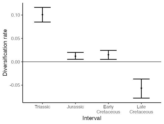
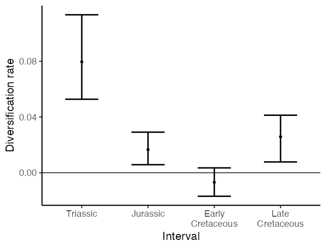
We can plot our skyline as error bars, with a discrete bar showing the range of estimated diversification rates in each time interval.
#Plot diversification skyline as error bars
ggplot(data = diversification_data, aes(x = interval, y = median, ymin = lower,
                             ymax = upper)) +
  geom_point(size = 1.5) +
  geom_errorbar(linewidth = 1, width = 0.5) +
  scale_colour_manual(values = c("black")) +
  geom_hline(aes(yintercept = 0), colour = "black") +
  scale_x_discrete(labels = function(x) str_wrap(x, width = 10)) +
  labs(x = "Interval", y = "Diversification rate") +
  theme_classic(base_size = 17)
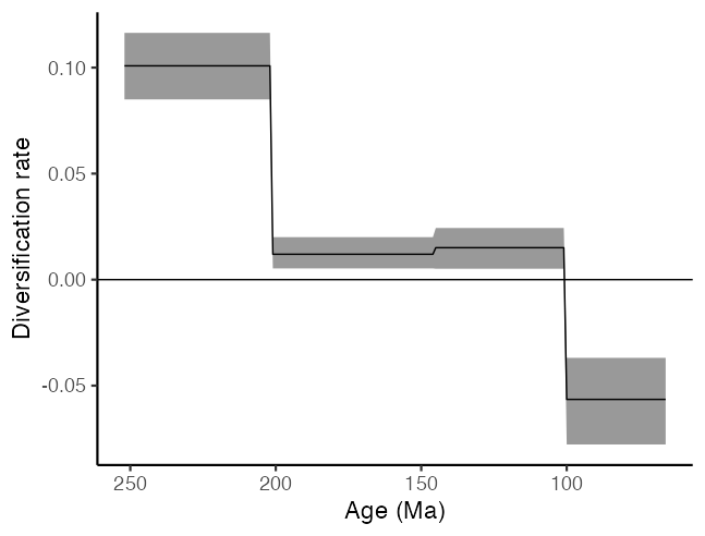
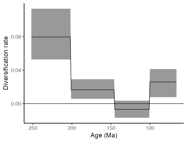
Alternatively, by extending our estimates across the temporal duration of each time interval, we can plot the diversification rate over time as a piecewise constant skyline.
#Plot diversification skyline as a ribbon plot
ages <- seq.int(252, 66)
interval <- c(rep("Triassic", ((252 - 202) + 1)),
              rep("Jurassic", ((201 - 146) + 1)),
              rep("Early Cretaceous", ((145 - 101) + 1)),
              rep("Late Cretaceous", ((100 - 66) + 1)))
age_table <- as.data.frame(cbind(ages, interval))
to_plot <- left_join(age_table, diversification_data, by = "interval")
to_plot$ages <- as.numeric(to_plot$ages)

ggplot(to_plot) +
  geom_ribbon(aes(x = ages, ymin = lower, ymax = upper), alpha = 0.5) +
  geom_line(aes(x = ages, y = median)) +
  scale_x_reverse() +
  geom_hline(aes(yintercept = 0), colour = "black") +
  xlab("Age (Ma)") + ylab("Diversification rate") +
  theme_classic(base_size = 17)
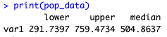
We can also investigate the other parameter estimated in the model, the estimated effective population size at the start of the coalescent process (which is the youngest end of our time interval). This estimate is a measure of the total species diversity of non-avian dinosaurs just before the Cretaceous-Paleogene boundary (although, as mentioned before, under the assumption of a Wright-Fisher population, so this value should be interpreted with caution). Again, we can calculate the median and 95% HPD values for our diversity estimate.
#Select estimated species diversity at end of time interval
population <- pull(coalescent, "ePopSize")

#Tell coda that this is an mcmc file, and calculate 95% HPD values
pop_mcmc <- as.mcmc(population)
pop_data <- as.data.frame(HPDinterval(pop_mcmc))

#Add median values to data frame
pop_data$median <- median(population)

#Display estimated species diversity and HPDs
print(pop_data)
The Fossilised-Birth-Death model results
We can now examine the results of our fossilised-birth-death model. Again, we need to read in the relevant log file and trim off the first 10% as burn-in.
# Navigate to Session > Set Working Directory > Choose Directory (on RStudio)
# or change file name to the full path to the log file
#(Use "dinosaur_BDSKY_final.log" if you used our pre-cooked XML)
fbd_file <- "dinosaur_BDSKY.log"

#Read in coalescent log and trim 10% burn-in
fbd <- read.table(fbd_file, header = T) %>% slice_tail(prop = 0.9)
We parameterised this model using birth, death and fossil sampling rates, so these are the parameters included in our log. However, our exponential coalescent model estimated diversification rates. If we want to make the fairest comparison between the two models, we should do so using the same parameters. Fortunately, it is straightforward to convert birth and death rates into diversification rates: simply, .
#Calculate diversification and turnover
birth_rates <- select(fbd, starts_with("birthRate"))
death_rates <- select(fbd, starts_with("deathRate"))

div_rates <- birth_rates - death_rates
colnames(div_rates) <- paste0("divRate.",
                              seq(1:ncol(div_rates)))
We can then calculate the median and 95% HPD values for our diversification estimates, just as we did before. This time, note that because the birth-death model runs from the origin forward-in-time, our “first” time bin is the oldest and our “fourth” time bin is the youngest. Even though we flipped the time direction of the break point times when setting up the XML file (using the reverseTimeArrays vector to change the direction of birthRateChangeTimes etc.), this has no effect on the order in which time bins are logged in the log file.
#Tell coda that this is an mcmc file, and calculate 95% HPD values
div_mcmc <- as.mcmc(div_rates)
div_data <- as.data.frame(HPDinterval(div_mcmc))

#Add median values to data frame
div_data$median <- apply(div_rates, 2, median)

#Add interval names
div_data$interval <- c("Triassic", "Jurassic", "Early Cretaceous",
                       "Late Cretaceous")
We can also use this same process to examine our fossil sampling rates.
#Select sampling estimates from log
samp_log <- select(fbd, starts_with("samplingBDS"))

#Tell coda that this is an mcmc file, and calculate 95% HPD values
samp_mcmc <- as.mcmc(samp_log)
samp_data <- as.data.frame(HPDinterval(samp_mcmc))

#Add median values to data frame
samp_data$median <- apply(samp_log, 2, median)

#Add interval names
samp_data$interval <- c("Triassic", "Jurassic", "Early Cretaceous",
                        "Late Cretaceous")
Once again, we will make sure that we specify the order of our time intervals.
#Ensure that the time intervals plot in the correct order
div_data$interval <- factor(div_data$interval,
                            levels = c("Triassic", "Jurassic",
                                       "Early Cretaceous", "Late Cretaceous"))

samp_data$interval <- factor(samp_data$interval,
                             levels = c("Triassic", "Jurassic",
                                        "Early Cretaceous", "Late Cretaceous"))
Again we have provided code so that the skylines can be plotted as discrete error bars…
ggplot(data = div_data, aes(x = interval, y = median, ymin = lower,
                                      ymax = upper)) +
  geom_point(size = 1.5) +
  geom_errorbar(linewidth = 1, width = 0.5) +
  scale_colour_manual(values = c("black")) +
  geom_hline(aes(yintercept = 0), colour = "black") +
  scale_x_discrete(labels = function(x) str_wrap(x, width = 10)) +
  labs(x = "Interval", y = "Diversification rate") +
  theme_classic(base_size = 17)

ggplot(data = samp_data, aes(x = interval, y = median, ymin = lower,
                            ymax = upper)) +
  geom_point(size = 1.5) +
  geom_errorbar(linewidth = 1, width = 0.5) +
  scale_colour_manual(values = c("black")) +
  geom_hline(aes(yintercept = 0), colour = "black") +
  scale_x_discrete(labels = function(x) str_wrap(x, width = 10)) +
  labs(x = "Interval", y = "Sampling rate") +
  theme_classic(base_size = 17)
…but also as piecewise constant skylines using ribbon plots.
ages <- seq.int(252, 66)
interval <- c(rep("Triassic", ((252 - 202) + 1)),
              rep("Jurassic", ((201 - 146) + 1)),
              rep("Early Cretaceous", ((145 - 101) + 1)),
              rep("Late Cretaceous", ((100 - 66) + 1)))
age_table <- as.data.frame(cbind(ages, interval))

div_plot <- left_join(age_table, div_data, by = "interval")
div_plot$ages <- as.numeric(div_plot$ages)
ggplot(div_plot) +
  geom_ribbon(aes(x = ages, ymin = lower, ymax = upper), alpha = 0.5) +
  geom_line(aes(x = ages, y = median)) +
  scale_x_reverse() +
  geom_hline(aes(yintercept = 0), colour = "black") +
  xlab("Age (Ma)") + ylab("Diversification rate") +
  theme_classic(base_size = 17)

samp_plot <- left_join(age_table, samp_data, by = "interval")
samp_plot$ages <- as.numeric(samp_plot$ages)
ggplot(samp_plot) +
  geom_ribbon(aes(x = ages, ymin = lower, ymax = upper), alpha = 0.5) +
  geom_line(aes(x = ages, y = median)) +
  scale_x_reverse() +
  geom_hline(aes(yintercept = 0), colour = "black") +
  xlab("Age (Ma)") + ylab("Sampling rate") +
  theme_classic(base_size = 17)
We can also examine the last parameter in our fossilised-birth-death model, which is the origin of the dinosaurian clade. Note that we add 66 to our estimates to account for the difference between the youngest tip (at the Cretaceous-Paleogene boundary) and the present day. If we didn’t add 66 to our estimates we would be estimating the duration of non-avian dinosaurs on Earth, instead of the time of their origin.
#Select origin data as an mcmc file, and calculate 95% HPD values
origin_mcmc <- as.mcmc(pull(fbd, "origin"))
origin_data <- as.data.frame(HPDinterval(origin_mcmc))

#Add median value to data frame
origin_data$median <- median(fbd$origin)

#Convert to time before present, rather than time before K-Pg boundary
origin_data <- origin_data + 66

#Display estimated origin and HPDs
print(origin_data)
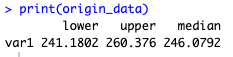
Our fossilised-birth-death model therefore suggests that dinosaurs originated around 246Ma, which would be during the Middle Triassic.
Model comparison
If we compare the skylines generated using our piecewise exponential growth coalescent and fossilised-birth-death models, we can see that they do not reconstruct the same diversification trajectory for dinosaurs across their evolutionary history. The piecewise exponential growth coalescent model indicates that the dinosaurs were experiencing negative diversification (net loss of species) during the Late Cretaceous, even prior to their total extinction at the Cretaceous-Paleogene boundary. In contrast, the fossilised-birth-death model suggests that the dinosaurs may have been in decline in the Early Cretaceous, but had returned to net diversification by the Late Cretaceous. One possible reason for this is that the fossilised-birth-death model includes fossil sampling rate as a parameter, whereas the exponential coalescent model simply assumes that there is no relationship between the sampling process and species richness, which may not be the case. Understanding the assumptions of the models we apply, and how well these assumptions fit our data, is therefore essential in Bayesian phylodynamics.
Useful Links
- Bayesian Evolutionary Analysis with BEAST 2 (Drummond & Bouckaert, 2014)
- BEAST 2 website and documentation: http://www.beast2.org/
- BEAST 1 website and documentation: http://beast.bio.ed.ac.uk
- Join the BEAST user discussion: http://groups.google.com/group/beast-users
Relevant References
- Bouckaert, R., Heled, J., Kühnert, D., Vaughan, T., Wu, C.-H., Xie, D., Suchard, M. A., Rambaut, A., & Drummond, A. J. (2014). BEAST 2: a software platform for Bayesian evolutionary analysis. PLoS Computational Biology, 10(4), e1003537. https://doi.org/10.1371/journal.pcbi.1003537
- Brusatte, S. L., Butler, R. J., Barrett, P. M., Carrano, M. T., Evans, D. C., Lloyd, G. T., Mannion, P. D., Norell, M. A., Peppe, D. J., Upchurch, P., & Williamson, T. E. (2015). The extinction of the dinosaurs. Biological Reviews, 90(2), 628–642. https://doi.org/10.1111/brv.12128
- Benson, R. B. J. (2018). Dinosaur macroevolution and macroecology. Annual Review of Ecology, Evolution, and Systematics, 49, 379–408. https://doi.org/10.1146/annurev-ecolsys-110617-062231
- Lloyd, G. T., Davis, K. E., Pisani, D., Tarver, J. E., Ruta, M., Sakamoto, M., Hone, D. W. E., Jennings, R., & Benton, M. J. (2008). Dinosaurs and the Cretaceous Terrestrial Revolution. Proceedings of the Royal Society B: Biological Sciences, 275(1650), 2483–2490. https://doi.org/10.1098/rspb.2008.0715
- Sakamoto, M., Benton, M. J., & Venditti, C. (2016). Dinosaurs in decline tens of millions of years before their final extinction. Proceedings of the National Academy of Sciences, 113(18), 5036–5040. https://doi.org/10.1073/pnas.1521478113
- Henao Diaz, L. F., Harmon, L. J., Sugawara, M. T. C., Miller, E. T., & Pennell, M. W. (2019). Macroevolutionary diversification rates show time dependency. Proceedings of the National Academy of Sciences, 116(15), 7403–7408. https://doi.org/10.1073/pnas.1818058116
- Stadler, T. (2009). On incomplete sampling under birth–death models and connections to the sampling-based coalescent. Journal of Theoretical Biology, 261(1), 58–66. https://doi.org/10.1016/j.jtbi.2009.07.018
- Brusatte, S. L., Nesbitt, S. J., Irmis, R. B., Butler, R. J., Benton, M. J., & Norell, M. A. (2010). The origin and early radiation of dinosaurs. Earth-Science Reviews, 101(1-2), 68–100. https://doi.org/10.1016/j.earscirev.2010.04.001
- Langer, M. C., Ezcurra, M. D., Bittencourt, J. S., & Novas, F. E. (2010). The origin and early evolution of dinosaurs. Biological Reviews, 85(1), 55–110. https://doi.org/10.1111/j.1469-185X.2009.00094.x
- Gavryushkina, A., Welch, D., Stadler, T., & Drummond, A. J. (2014). Bayesian Inference of Sampled Ancestor Trees for Epidemiology and Fossil Calibration. PLoS Computational Biology, 10(12), e1003919. https://doi.org/10.1371/journal.pcbi.1003919
- Drummond, A. J., & Bouckaert, R. R. (2014). Bayesian evolutionary analysis with BEAST 2. Cambridge University Press.
Citation
If you found Taming the BEAST helpful in designing your research, please cite the following paper:
Joëlle Barido-Sottani, Veronika Bošková, Louis du Plessis, Denise Kühnert, Carsten Magnus, Venelin Mitov, Nicola F. Müller, Jūlija Pečerska, David A. Rasmussen, Chi Zhang, Alexei J. Drummond, Tracy A. Heath, Oliver G. Pybus, Timothy G. Vaughan, Tanja Stadler (2018). Taming the BEAST – A community teaching material resource for BEAST 2. Systematic Biology, 67(1), 170–-174. doi: 10.1093/sysbio/syx060