
Background
In this tutorial we will analyse 100 full genome sequences from the 2009 H1N1 flu pandemic in North America. The sequences were collected from about February to November, such that their sampling times can be used for calibration. They were analysed by Hedge and Rambaut (Hedge et al., 2013). An important aspect of using sampling times for calibration is that the sampling time should capture a sufficient number of substitutions, i.e. the population should be measurably evolving (Drummond et al., 2003). One way to verify whether a population is measurably evolving is to compare the prior and posterior distribution of the tree height, which we will do here. We will also use a relaxed molecular clock and the bModel test add-on to average over substitution models (Bouckaert & Drummond, 2017). In the optional exercises we can compare the estimates from a relaxed molecular clock to those from a strict molecular clock model. In a subsequent tutorial we will use the exponential coalescent and constant birth-death model to infer epidemiological parameters.
Programs used in this Exercise
BEAST2 - Bayesian Evolutionary Analysis Sampling Trees 2
BEAST2 is a free software package for Bayesian evolutionary analysis of molecular sequences using MCMC and strictly oriented toward inference using rooted, time-measured phylogenetic trees (Bouckaert et al., 2014). This tutorial uses the BEAST2 version 2.5.
bModelTest
bModelTest (Bouckaert & Drummond, 2017) is used to average over substitution models during the MCMC. For installation instructions click here.
BEAUti2 - Bayesian Evolutionary Analysis Utility
BEAUti2 is a graphical user interface tool for generating BEAST2 XML configuration files.
Both BEAST2 and BEAUti2 are Java programs, which means that the exact same code runs on all platforms. For us it simply means that the interface will be the same on all platforms. The screenshots used in this tutorial are taken on a Mac OS X computer; however, both programs will have the same layout and functionality on both Windows and Linux. BEAUti2 is provided as a part of the BEAST2 package so you do not need to install it separately.
TreeAnnotator
TreeAnnotator is used to summarise the posterior sample of trees to produce a maximum clade credibility tree. It can also be used to summarise and visualise the posterior estimates of other tree parameters (e.g. node height).
TreeAnnotator is provided as a part of the BEAST2 package so you do not need to install it separately.
Tracer
Tracer (http://tree.bio.ed.ac.uk/software/tracer) is used to summarize the posterior estimates of the various parameters sampled by the Markov Chain. This program can be used for visual inspection and to assess convergence. It helps to quickly view median estimates and 95% highest posterior density intervals of the parameters, and calculates the effective sample sizes (ESS) of parameters. It can also be used to investigate potential parameter correlations. We will be using Tracer v1.7.
IcyTree
IcyTree (https://icytree.org) is a browser-based phylogenetic tree viewer (Vaughan, 2017). It is intended for rapid visualisation of phylogenetic tree files. It can also render phylogenetic networks provided in extended Newick format. IcyTree is compatible with current versions of Mozilla Firefox and Google Chrome.
Setting up the BEAST2 xml
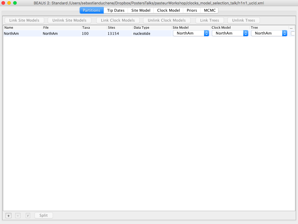
BEAST2 requires the data and model specified in an xml format, which can be done using the program BEAUti. Open BEAUti and drag the alignment (NorthAm.Nov.fasta) to this window Figure 1. Note that there are several tabs (Partitions, Tip Dates, Site Model, Clock Model, Priors, and MCMC).
Click on the Tip Dates tab and check the box Use tip dates Figure 2.
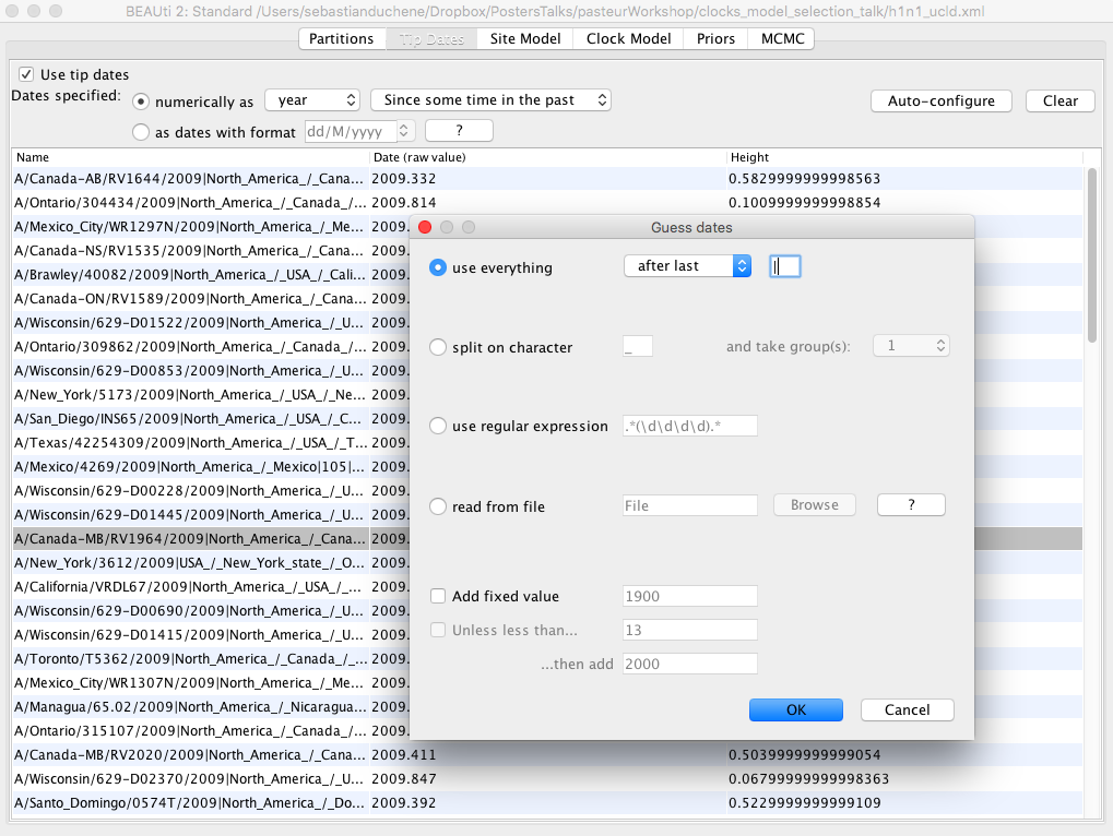
| To use the tip dates as calibrations, click on the Auto-configure button. Check the first box (use everything) and in the dropdown menu, select after last, and type in a vertical line ( | ) as shown in Fig 2. |
The BEAUti window should now display the dates for each of the sequences under the column date.
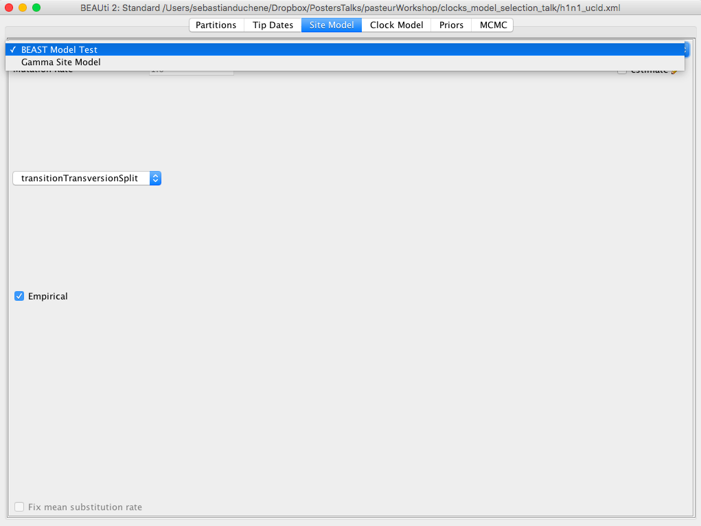
Click on the Site Model tab. Instead of using a single substitution model, we will average over those that account for differences in the number of transitions to transversions. In the first drop-down menu select BEAST Model Test. There is a second drop-down menu to select the range of models that we will sample during the MCMC. Select transitionToTransversionSpit to limit our search to those that allow for differences in transitions to transversions. Click on the box Empirical to use the empirical base frequencies. These options should look like those in Figure 3.
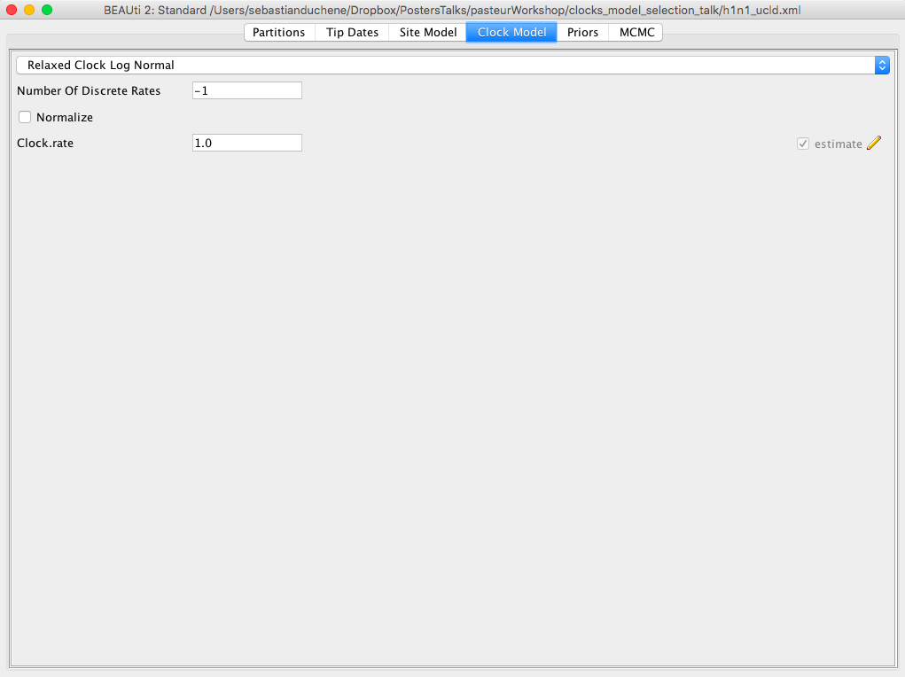
Click on the Clock Model tab. In the dropdown menu, select Relaxed Clock Lognormal Figure 4. The other default options are fine.
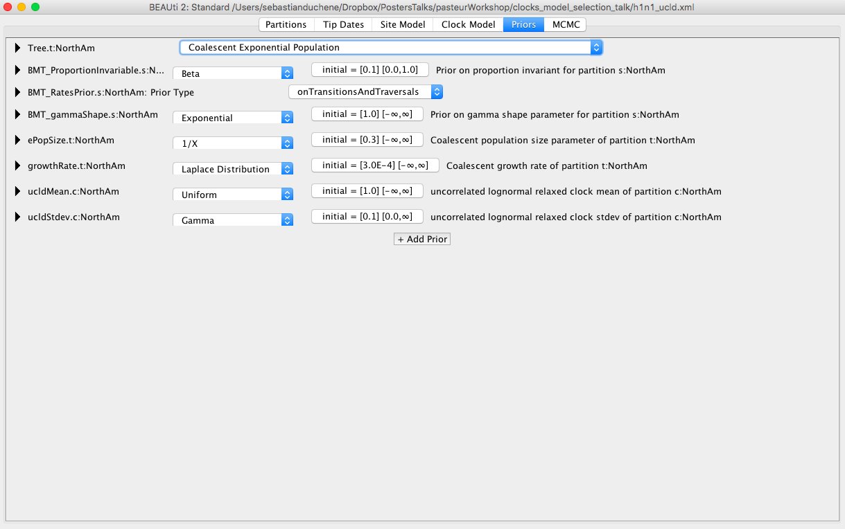
Click on the Priors tab. Select the Coalescent Exponential Population model Figure 5. Most of the remaining priors are fine for our analyses, but it is a good exercise to inspect these distributions. In particular, set a Uniform distribution for the mean of the lognormal distribution for the rate with lower and upper bounds of 0 and 1, respectively. This is based on our knowledge that flu probably does not evolve at a rate that is faster than 1 subs/site/year.
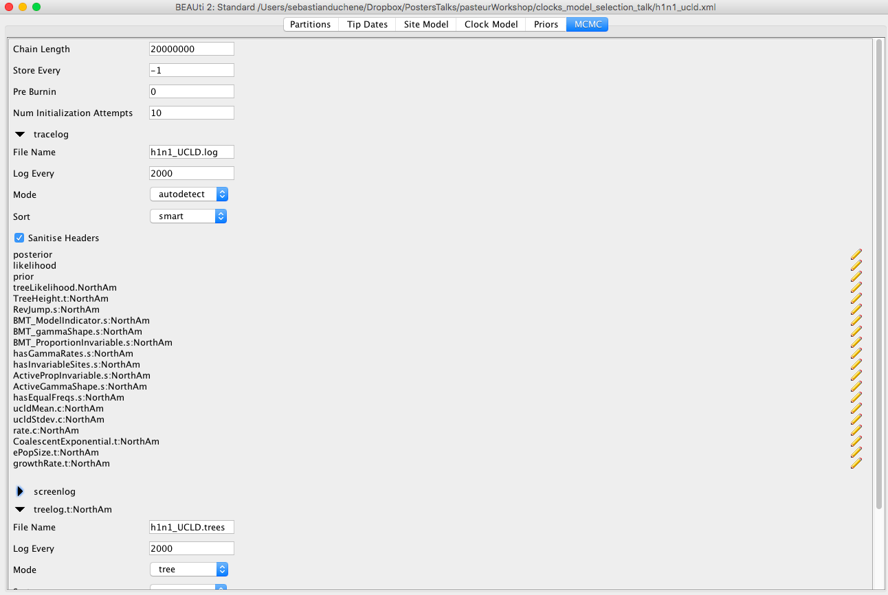
Click on the MCMC tab. Here, we can select different options for the MCMC. The chain length should be 20000000. Click on tracelog and treelog to specify the BEAST output, which is a set of trees and parameters values, sampled from the posterior. Ensure that the Log Every box is 2000 for the trees and log files. Name the log and tree files h1n1_UCLD.log and h1n1_UCLD.trees, respectively Figure 6. We use the extension _ucld to refer to the uncorrelated lognormal clock model.
Our BEAST input file is ready. To save it, click on File, Save, and name it h1n1_ucld.xml. Do not close BEAUti.
Running the analysis
To run BEAST, double-click on the BEAST2 icon. A window with some options will appear Figure 7.
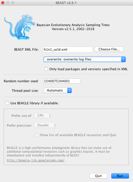
Click on Choose File… and select the xml file that we created in BEAUti. Click Run. The MCMC will start running Figure 8.
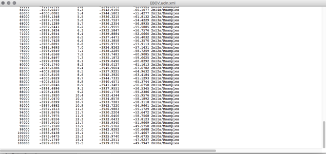
Note that two files have been created in the folder where we saved the xml file, these are the .trees and .log files. This analysis can take up to two hours to complete, but we can inspect the log file much earlier.
Analyzing the results
After letting BEAST run for about 30 minutes open Tracer Figure 9, and drag the h1n1_UCLD.log file to the right pane of the Tracer window.
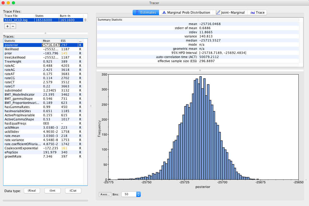
Select the Trace tab. This shows how the MCMC has sampled in parameter space.
Question: Inspect the trace for TreeHeight, and the clock model parameters (rate.mean and rate.variance). Does it appear that we have sufficient sampling from the stationary distribution? What do these parameters mean?
An other diagnostic of MCMC sampling is the effective sample size, shown in Tracer as ESS. This is the estimated number of independent samples obtained. A rule of thumb is to ensure that ESS is at least 200 for all parameters.
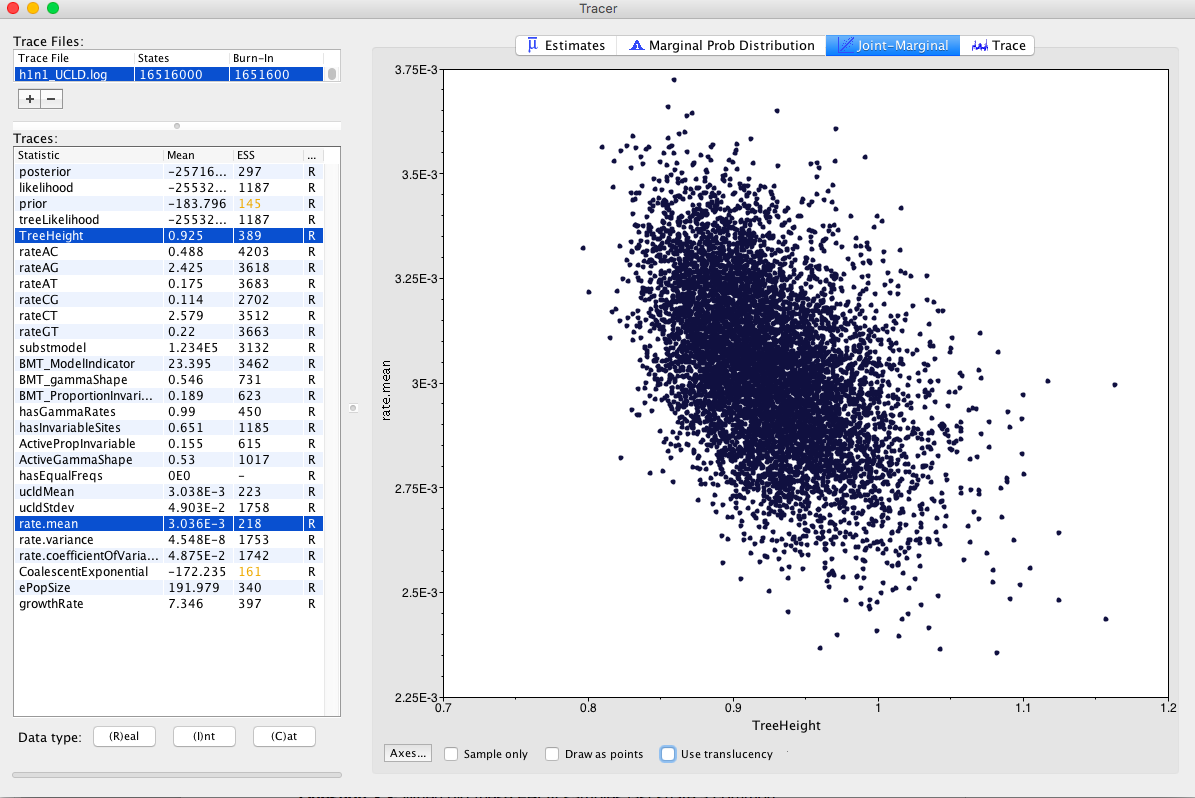
Select the TreeHeight and rate.mean parameters (you might need to use the command or control key to select them at the same time), then select the Joint-marginal tab. TreeHeight is the age of the root of the tree, while rate.mean is the mean substitution rate in the model. If these parameters were independent, we would expect them to form a cloud along the x and y axes. However, these two parameters are naturally correlated. In particular, high rates typically lead to more recent timescales for the root, while lower rates lead to older root ages Figure 10.
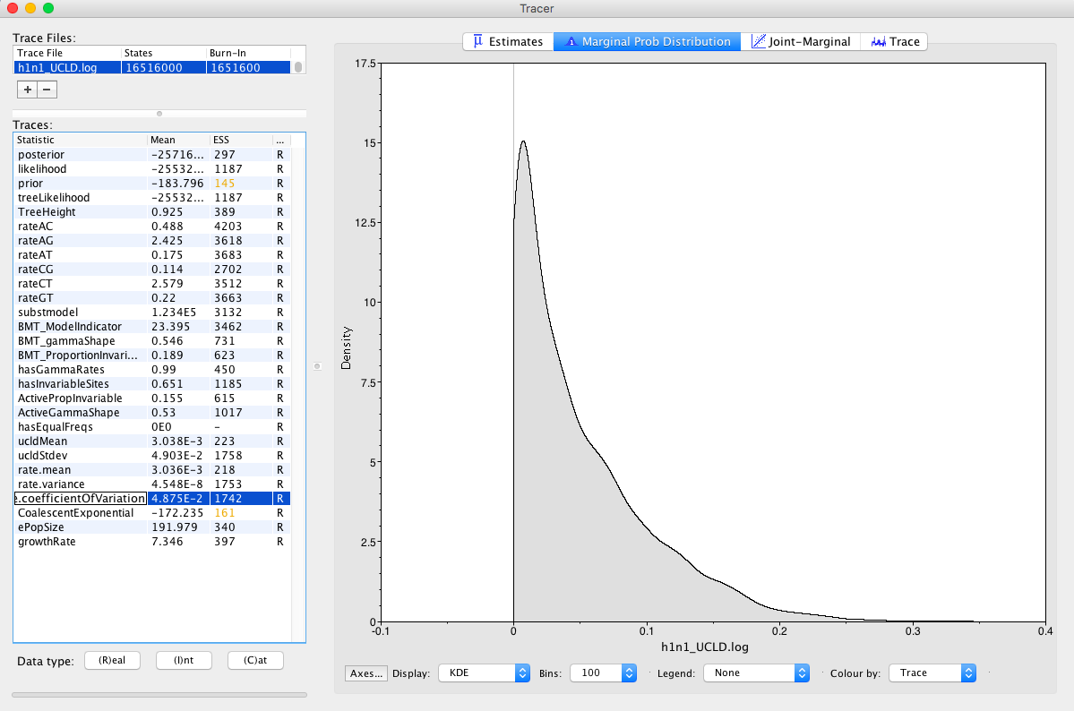
Check rate.coefficientOfVariation parameter Figure 11. This is the standard deviation of branch rates divided by the mean rate. Typically, if this parameter is abutting zero, the data have low rate variation, such that they can follow a strict clock.
Question: Does this data set appear to follow a strict clock, or does it display substantial rate variation among lineages?
Question: When did these h1n1 samples last share a common ancestor? Is it consistent with our knowledge of the 2009 pandemic?
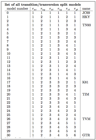
Select the BMT_ModelIndicator trace. These are the models that were sampled using an index as shown in Figure 12.
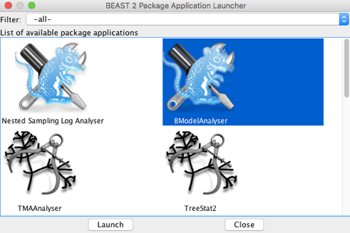
Optional exercise: The BEAST2 app BModelAnalyser provides a visual inspection of substitution model averaging. To use it, open the BEAST2 folder and find the AppLauncher icon. Click it to obtain a list of BEAST2 apps (Figure 13).
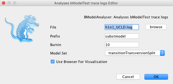
Select BModelAnalyser and click Launch. A window will pop up with a few options. Click on browse and find the log file for the h1n1 data and set the remaining options as shown in Figure 14.
Click OK. A browser with a figure similar to Figure 15 should appear in your default browser.
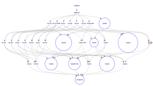
Question: Which model has the highest posterior probability? Does this model include among site rate heterogeneity? (hint: check the hasGammaRates and hasInvariableSites traces)
The .trees file contains trees sampled from the posterior. We can summarise them by using TreeAnnotator, which is distributed with the BEAST package. Double-click the TreeAnnotator icon. The window in Figure 16 will appear.
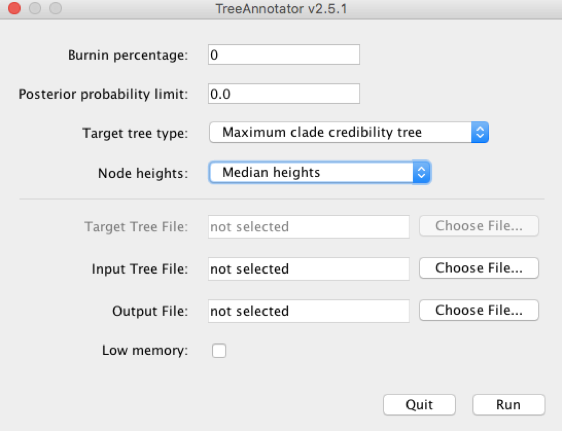
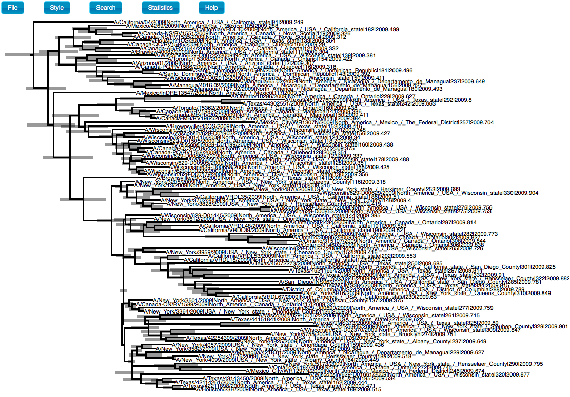
Type 10 for Burnin percentage and choose the same settings for Target tree type and node heights as shown in Figure 16. In Input Tree File click on Choose File…, and select h1n1_ucld.trees. In Output File click on Choose File… and type h1n1_ucld.tre. Note that we use the .tre extension for the output file. Click on Run. After the program has run, find the h1n1_ucld.tre and open it in icytree. Click on Style, Node-height error bars, and select height_95%-HPD (Figure 17).
Optional exercise 1
Use the BEAUti window, which we left open, to sample from the prior distribution. This is useful to assess whether the data are informative about parameters of interest. To do this, go to the MCMC tab and tick the SampleFromPrior box. Change the names of the output log and trees files to h1n1_ucld_prior.log and h1n1_ucld_prior.trees and go to File, Save as, and save it as h1n1_UCLD_prior.xml. This analysis will run much faster because it does not need to calculate the phylogenetic likelihood. After it has run, load the log file with that from the posterior.
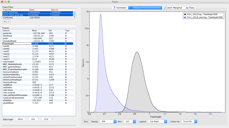
Question: Does it seem like our data are driving our estimates of evolutionary rates and timescales (hint: compare the prior and the posterior for the tree height, as in Figure 18, and for the rate.mean parameters).
Optional exercise 2
Use the BEAUti window, which we left open, to set up a strict clock. To do this go to the Clock Model tab and select Strict Clock. In the MCMC tab change the output file names to h1n1_sc.log, h1n1_sc.trees. Save it as h1n1_sc.xml and run it in BEAST. Compare the rate and node age estimates to those from the relaxed clock used here.
Relevant References
- Hedge, J., Lycett, S. J., & Rambaut, A. (2013). Real-time characterization of the molecular epidemiology of an influenza pandemic. Biology Letters, 9(5), 20130331.
- Drummond, A. J., Pybus, O. G., Rambaut, A., Forsberg, R., & Rodrigo, A. G. (2003). Measurably evolving populations. Trends in Ecology & Evolution, 18(9), 481–488.
- Bouckaert, R. R., & Drummond, A. J. (2017). bModelTest: Bayesian phylogenetic site model averaging and model comparison. BMC Evolutionary Biology, 17(1), 42.
- Bouckaert, R., Heled, J., Kühnert, D., Vaughan, T., Wu, C.-H., Xie, D., Suchard, M. A., Rambaut, A., & Drummond, A. J. (2014). BEAST 2: a software platform for Bayesian evolutionary analysis. PLoS Computational Biology, 10(4), e1003537. https://doi.org/10.1371/journal.pcbi.1003537
- Vaughan, T. G. (2017). IcyTree: rapid browser-based visualization for phylogenetic trees and networks. Bioinformatics, 33(15), 2392–2394.
Citation
If you found Taming the BEAST helpful in designing your research, please cite the following paper:
Joëlle Barido-Sottani, Veronika Bošková, Louis du Plessis, Denise Kühnert, Carsten Magnus, Venelin Mitov, Nicola F. Müller, Jūlija Pečerska, David A. Rasmussen, Chi Zhang, Alexei J. Drummond, Tracy A. Heath, Oliver G. Pybus, Timothy G. Vaughan, Tanja Stadler (2018). Taming the BEAST – A community teaching material resource for BEAST 2. Systematic Biology, 67(1), 170–-174. doi: 10.1093/sysbio/syx060