


Background
This tutorial will show how to configure and run a model with lineage-dependent birth and death rates, using the BEAST2 package MSBD.
The MSBD package relies on a multi-type birth death model which is composed of a number of evolutionary regimes, also called types or states, .
Each type is associated with a birth rate and a death rate . A lineage in type will change to any another type with a uniform rate , where is the total type change rate. The MSBD package is able to infer , and and for all types, as well as the locations of types and type changes on the tree.
More details on the model and an evaluation of its performance in various conditions can be found in the original publication (Barido-Sottani et al., 2020).
You may notice similarities between MSBD and the model used in another BEAST2 package, BDMM. The main difference is that MSBD is able to infer the number of types as well as the types at the tips of the tree, whereas BDMM requires you to fix them. Thus MSBD is more appropriate if the character driving the differences in rates is unobserved or unknown. On the other hand, BDMM integrates more complex dynamics than the current implementation of MSBD: in particular, it includes asymmetrical transition rates as well as mixed birth events (where the two lineages produced by a birth event are of different types), which are not currently available in MSBD.
Programs used in this Exercise
BEAST2 - Bayesian Evolutionary Analysis Sampling Trees 2
BEAST2 is a free software package for Bayesian evolutionary analysis of molecular sequences using MCMC and strictly oriented toward inference using rooted, time-measured phylogenetic trees (Bouckaert et al., 2014). This tutorial uses BEAST2 version 2.7.4.
BEAUti – Bayesian Evolutionary Analysis Utility
BEAUti is a utility program with a graphical user interface for creating BEAST2 input files, which are written in XML. The eXtensible Markup Language (XML) is a general-purpose markup language, which allows for the combination of text and additional information. The use of the XML makes analysis specification very flexible and readable by both the program and people. The XML file specifies all the components of the analysis, including sequences, node calibrations, models, priors, output file names.
TreeAnnotator
TreeAnnotator is used to summarize the posterior sample of trees to produce a maximum clade credibility tree and summarize the posterior estimates of other parameters that can be easily visualized on the tree (e.g. node height). This program is also useful for comparing a specific tree topology and branching times to the set of trees sampled in the MCMC analysis.
Tracer
Tracer is used for assessing and summarizing the posterior estimates of the various parameters sampled by the Markov Chain. This program can be used for visual inspection and assessment of convergence and it also calculates 95% credible intervals (which approximate the 95% highest posterior density intervals) and effective sample sizes (ESS) of parameters. Contrary to the other software in this section, Tracer is not distributed with BEAST2 and needs to be downloaded separately here.
Practical: Lineage-specific Birth and Death Rate Inference
Dataset: Hummingbird Phylogeny
The dataset used in this tutorial is a time-calibrated phylogeny of 284 species of hummingbirds, which was estimated by (McGuire et al., 2014). This phylogeny was built from an alignment of 436 sequences representing six genes (four nuclear and two mitochondrial).
In this tutorial, we focus on estimating the MSBD model and its parameters, and so we are going to fix this phylogeny in our analysis. However, it is also possible to co-estimate both the phylogeny and the MSBD model from an alignment in BEAST2.
Setting up the XML file
This section will demonstrate how to create an XML configuration file using BEAUti, which will then be used to run the analysis in BEAST2.
Package installation
The first step is to install the MSBD package, which will allow us to set up and run an analysis with lineage-specific birth and death rates.
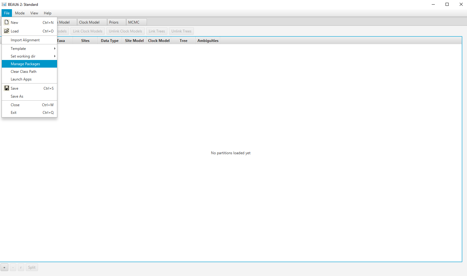
Open the BEAST2 Package Manager by navigating to File > Manage Packages. (Figure 1)
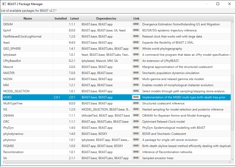
Install the MSBD package by selecting it and clicking the Install/Upgrade button. (Figure 2)
BEAUti needs to be restarted for the newly installed package to be loaded properly.
Close the BEAST2 Package Manager and restart BEAUti to fully load the MSBD package.
Setting the templates
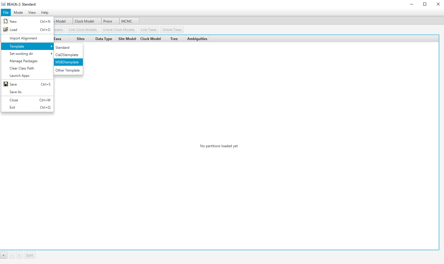
BEAUti uses templates to define specific model configurations. The MSBD template needs to be selected to set up an analysis using the MSBD model.
Select the MSBD template by navigating to File > Template. (Figure 3)
Importing the alignment
This analysis will be run with a fixed tree topology, however BEAUti requires an alignment to be loaded in order to set the other components of the model. As a result, we will load a dummy alignment, which is just the sequence “A” for all taxa.
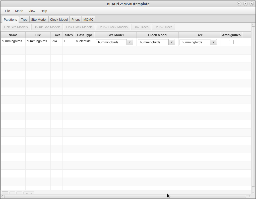
In the Partitions panel, import the alignment by navigating to File > Import Alignment in the menu (Figure 4) and then finding the
hummingbirds.nexfile on your computer or simply drag and drop the file into the BEAUti window.
Importing the tree
As mentioned earlier, we want to run this analysis with a fixed tree topology. First, we need to specify that our tree is fixed and will not be changed during the inference.
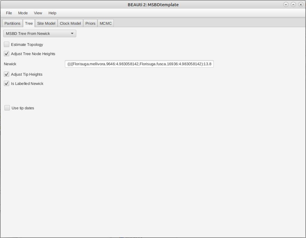
In the Tree panel, uncheck the Estimate Topology checkbox.
Then we need to actually provide the tree to use. By default BEAUti generates a random starting tree compatible with the alignment, so we need to change this to our fixed tree.
In the Starting Tree panel, set the dropdown to Tree From Newick. Copy-paste the Newick tree found in the
hummingbirds_initial_tree.trefile into the Newick field.
The final tree configuration is shown in Figure 5.
The parameter priors
The next step is to look at the parameter priors, in the Priors panel. The default priors on the birth rates (), death rates () and total number of types () are reasonable for this dataset so we will not change them.
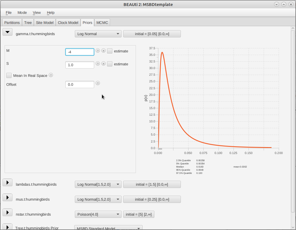
The expected average number of type changes across the entire tree is given by , where L is the total length of the tree. The length of the fixed tree used in this analysis is , so the default prior on would lead to a high expected number of type changes. From the previous analysis performed in BAMM, we expect only a few type changes across this phylogeny, so we will set the prior on to a lower range, using a LogNormal(-4.0, 1.0) distribution.
Click on the arrow next to gamma and change the value for M (mean) of the default log normal distribution to -4 (Figure 6).
The tree prior
Next, we will specify the tree prior, i.e. the MSBD model. By default most of the parameters of the model are estimated, so it is not necessary to change their starting values. However, the extant sampling proportion () and extinct sampling probability () are fixed. There are no extinct samples in this dataset, and we have sampled 86% of the extant hummingbirds species so we will set and .
Click on the arrow next to Tree and change the value for rho (extant sampling proportion) of the MSBD model to 0.86 (Figure 7).
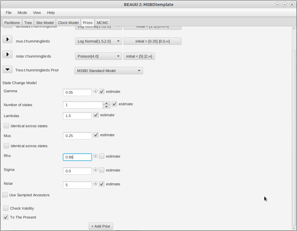
Note that many other options are available in this section, such as fixing the number of states or the value of some parameters (estimate checkboxes), setting the birth rate or the death rate to be shared between states (identical across states checkboxes), or setting the model to only use sampling-through-time (To The Present checkbox) .
MCMC options
The next step is to set the options for running the chain, in the MCMC panel. We can see that several loggers are set by default:
- the regular trace log, which in our case only records the posterior, likelihood and prior, as we are not using a substitution or clock model.
- the screenlog, which shows the advancement of the chain to the screen.
- the tree log, which will log the trees in Nexus format, with the birth and death rate on each edge as metadata.
- the state change model log, which logs the parameters associated with the model, i.e. , , the number of sampled states and the birth and death rates for each state ( and ).
- the tip rates log, which logs the birth and death rates at each tip (optionally, at each node if the nodeLog option is activated).
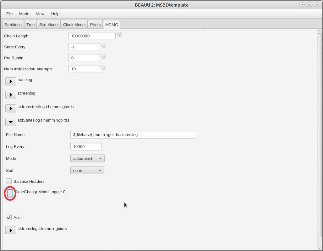
These last three logs are specific to MSBD. The only thing we will change here is the number of states recorded in the model. By default, only the sampled states are recorded, however this results in a log that is not in table format and so cannot be easily loaded into Tracer. Fixing the number of recorded states solves this problem.
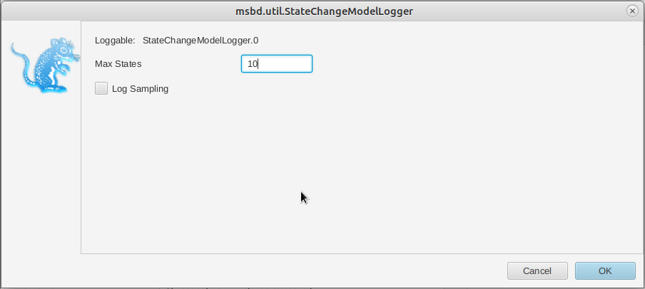
In the MCMC panel, click on the arrow next to stdStateslog and click on the Edit button to the right of the StateChangeModelLogger (Figure 8).
In the new panel, set the value of maxStates to 10 (Figure 9). Close the panel by clicking on OK.
Once all the options have been set, the final step is to save the XML.
Save the XML file as
hummingbirds.xmlby navigating to File > Save.
Running the analysis in BEAST2
Start BEAST2 and choose the file
hummingbirds.xml.If you have BEAGLE installed tick the box to Use BEAGLE library if available, which will make the run faster.
Hit Run to start the analysis.
The run should take about 15-20 minutes.
Analyzing the output
Output files
Our run has generated 4 different files:
hummingbirds.logwhich is the general trace log.hummingbirds.hummingbirds.states.logwhich recorded the parameters associated with the state model.hummingbirds.hummingbirds.rates.logwhich recorded the rates on tips of the tree.hummingbirds.hummingbirds.rates.treeswhich recorded the sampled trees in Nexus format.
Analyzing the log files
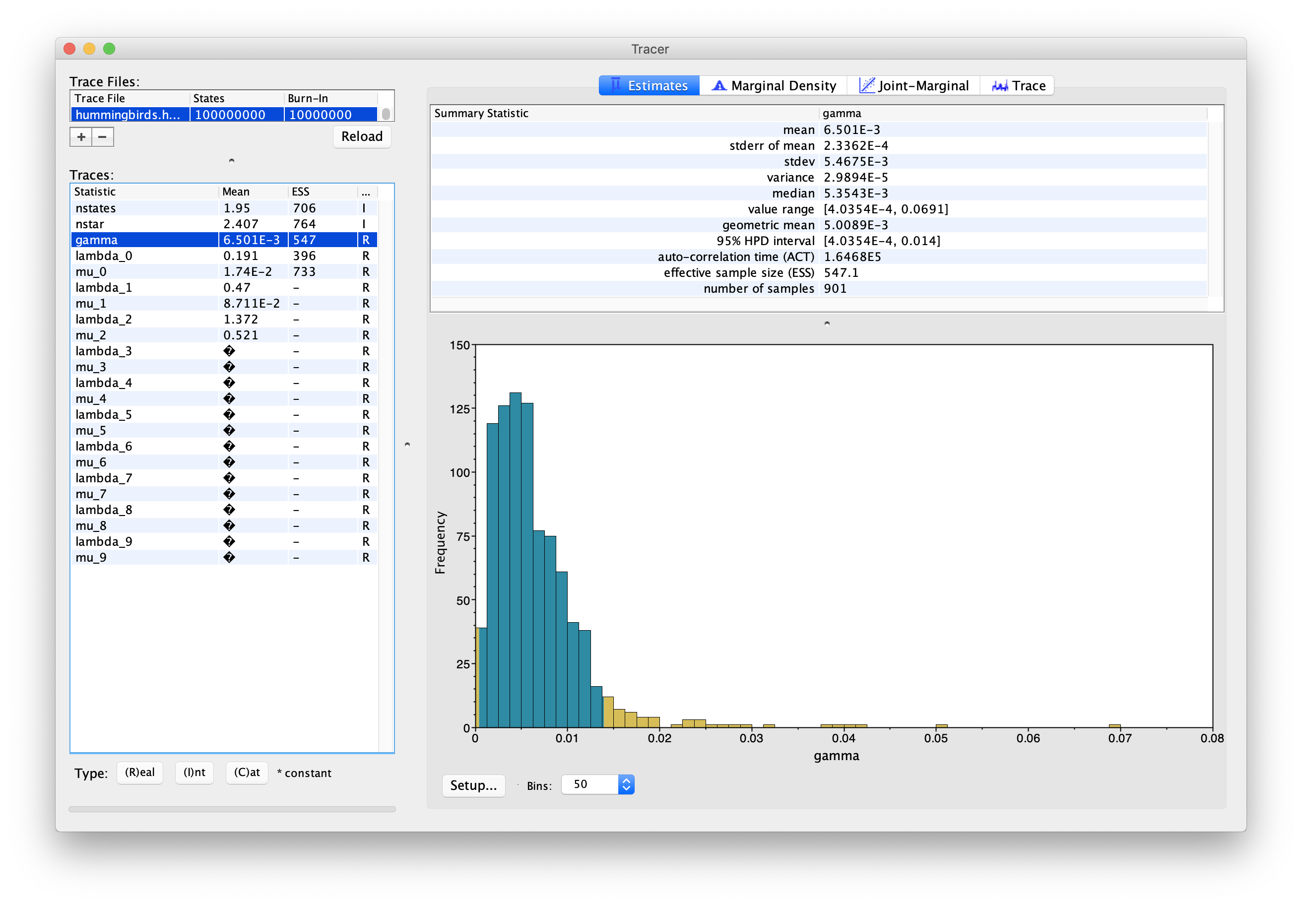
We will use the software Tracer to analyze the log files. The general trace log is not very interesting in our case, as we used a fixed tree. Next, we will look at the MSBD model log, contained in the file hummingbirds.hummingbirds.states.log.
Figure 10 shows the estimated posterior distribution for the type change rate, which in this analysis has a median estimate of 5.35E-3, with a 95% HPD of [4.04E-4 ; 0.014].
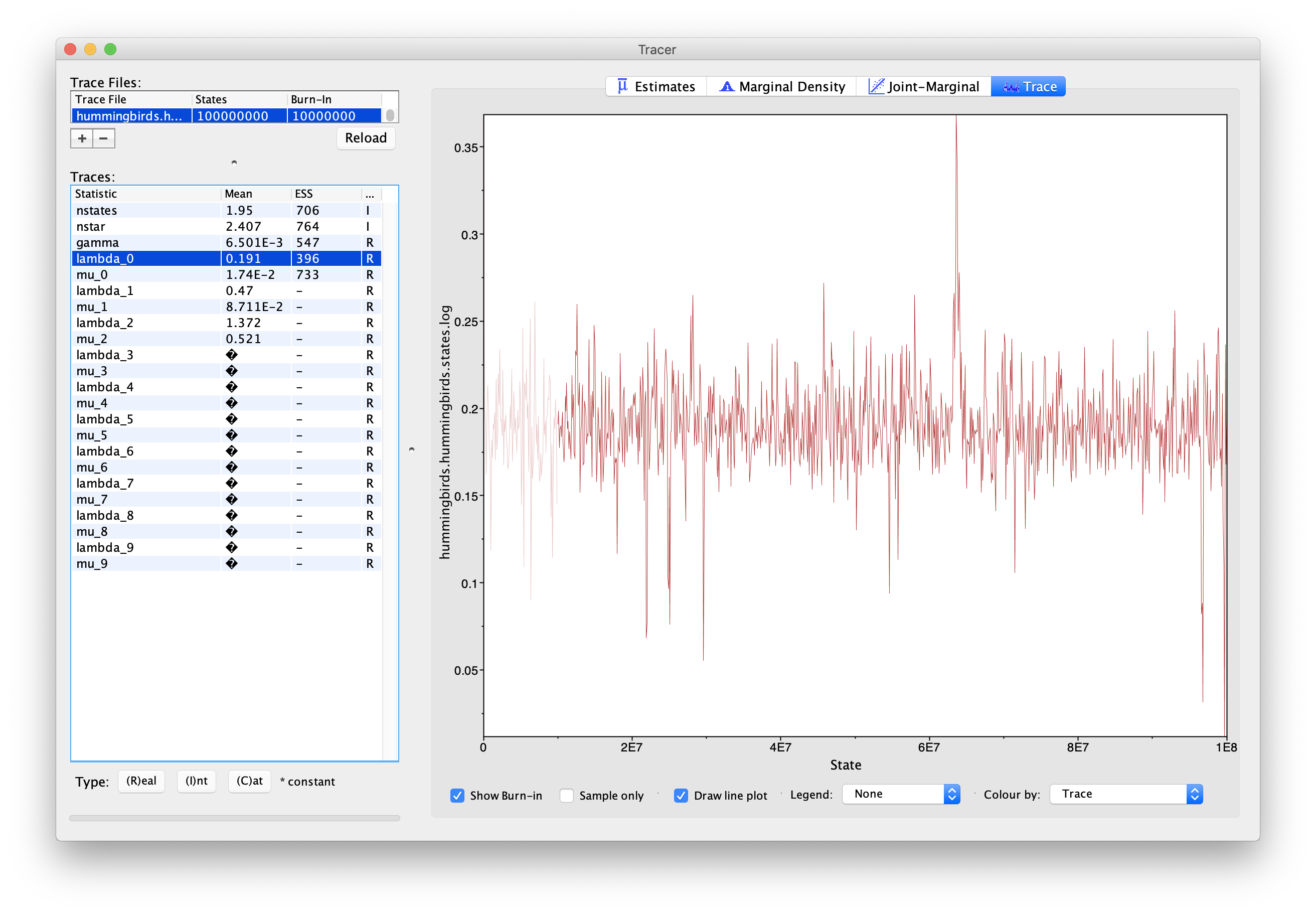
One important thing to note is that the estimates of lambda and mu in this log should not be directly used. This is due to the fact that the types in our model are not tied to tips, so they may not represent the same evolutionary regimes in all samples. For instance, in the presence of two regimes, there may be samples where type 0 corresponds to the regime with higher birth, while in other samples this regime is represented by type 1. We can see this in Figure 11, where the estimate for lambda_0 shows a discrepancy around 6.5E7 samples, which corresponds to lambda_0 and lambda_1 exchanging values. This also means that ESS values for these parameters may be low even if the chain has converged.
In order to look at the actual birth and death rates estimates, we can look at the tip rates log, stored in the file hummingbirds.hummingbirds.rates.log. Figure 12 and Figure 13 show examples of the estimated posterior distributions of the birth rate for two different tips.
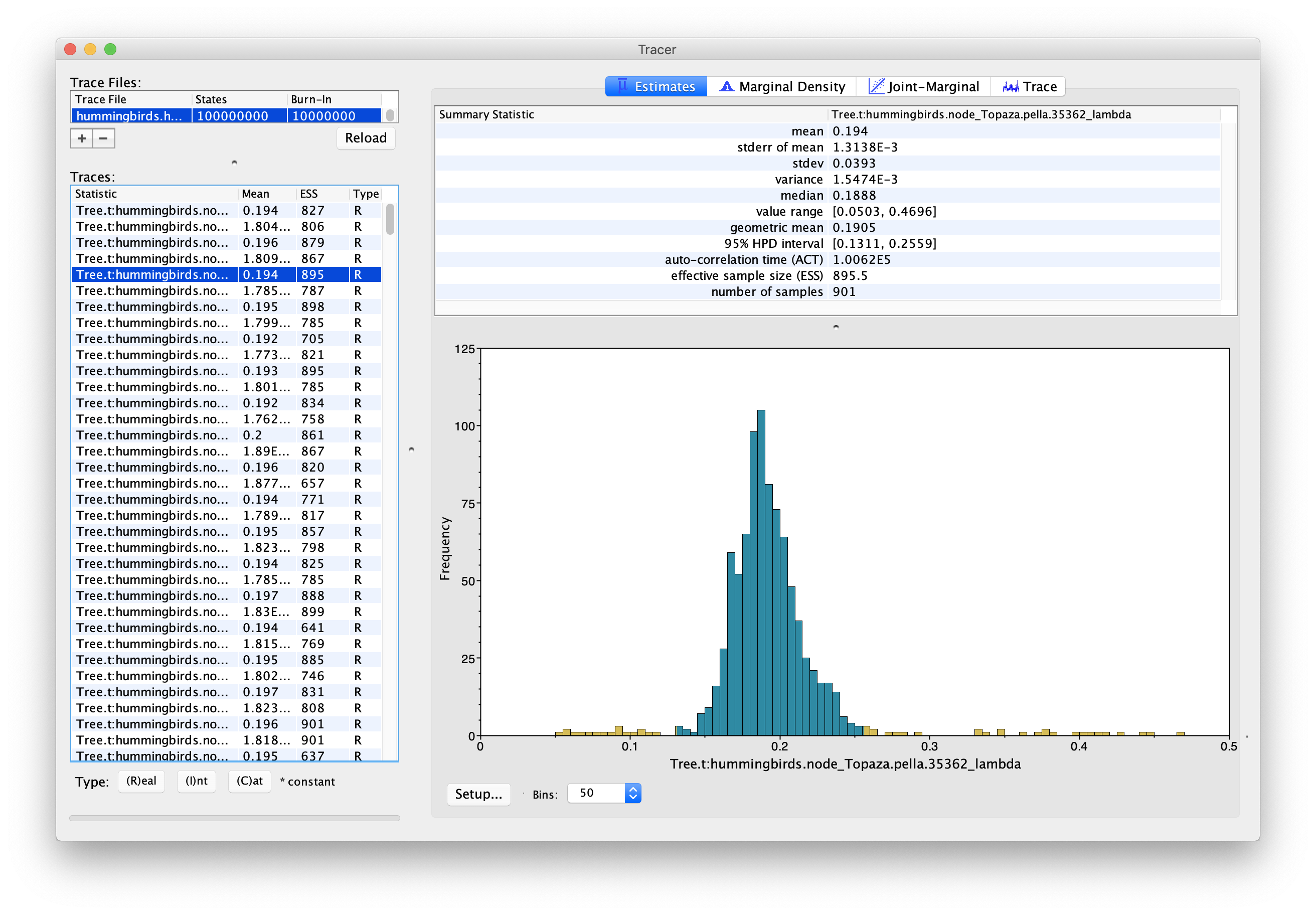
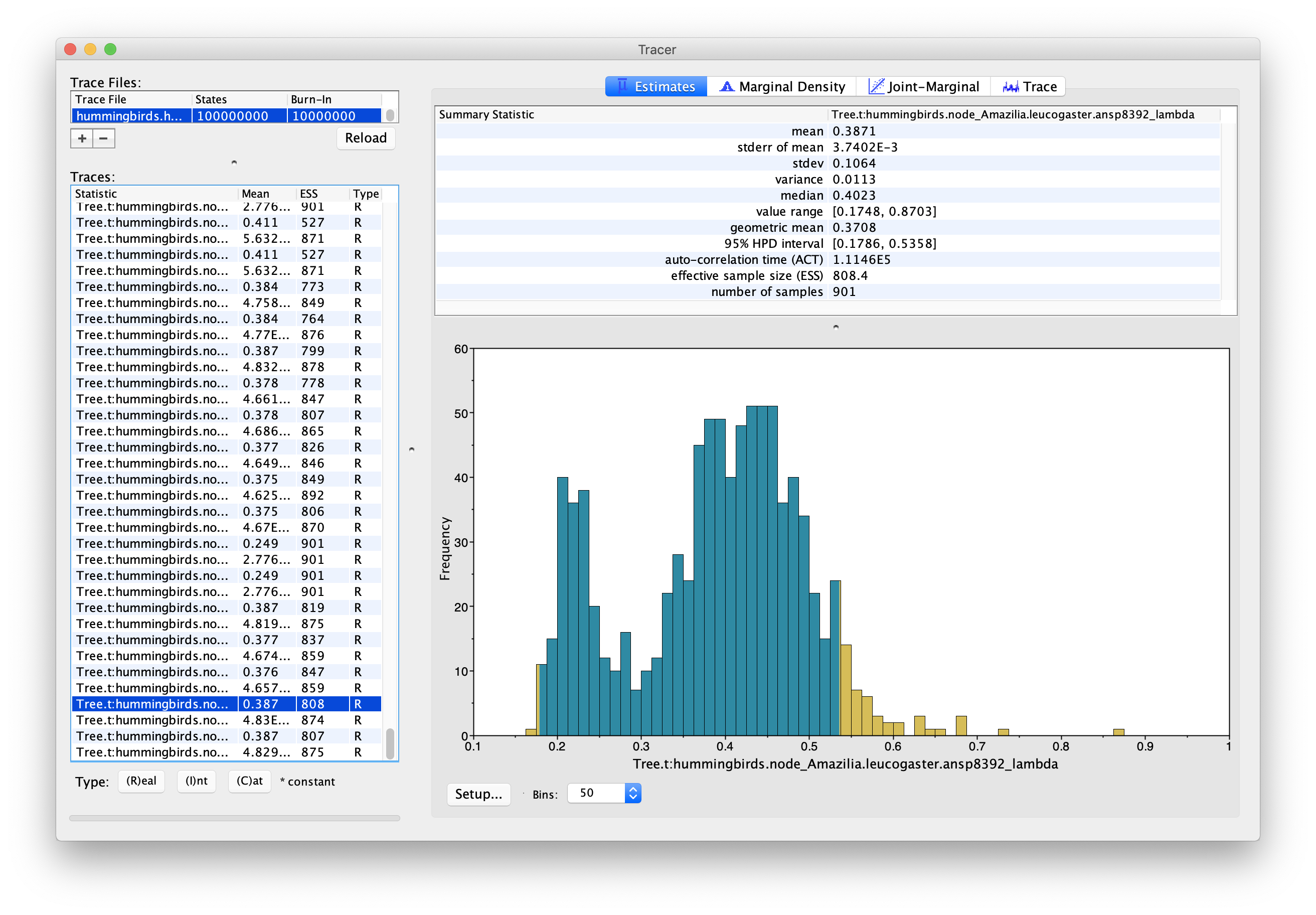
We can see that these two tips present two very different configurations. The first tip shows a unimodal posterior distribution, which indicates that it is confidently assigned to one particular evolutionary regime. On the other hand, the second tip presents a bimodal distribution, indicating that there are two distinct evolutionary regimes, with two distinct birth rates, which it can be assigned to. This is important to note because the usual metrics used to summarize posterior distributions, i.e. the median and 95% HPD interval, work well in the first case but can give a misleading representation of the posterior in the second case. In this case the median estimate for the birth rate of Amazilia.leucogaster is 0.40, which corresponds approximately to the second mode of the distribution, however neither the median nor the 95% HPD interval show the existence of a second possible regime, with birth rate 0.22.
Analyzing the trees
Another way to visualize the results is to look at the rates as plotted on the tree. We can use TreeAnnotator to build an MCC tree from the tree log in the file hummingbirds.hummingbirds.rates.trees. Since we also logged the birth and death rates for each edge in the tree log, these parameters will also be summarized along with the tree.
Start TreeAnnotator and set the input tree to the tree file
hummingbirds.hummingbirds.rates.trees.Give a name to the output file, for instance
hummingbirds.MCC.tre.Finally, click Run to start the summary.
The MCC tree can be loaded into any tree visualization software, such as FigTree or IcyTree. We are going to use the R script provided in this tutorial plot_MCC.R. This script takes as input the MCC tree file and an output file to store the plot, and it will plot the MCC tree with edges coloured by the median estimates of the birth and death rates.
Run the following commands in an R console to create the plots:
source("plot_MCC.R")
MCC_colour_plot("hummingbirds.MCC.tre", plotfile = "hummingbirds_MCC.pdf")
Figure 14 and Figure 15 show the resulting plots for the birth rate and the death rate, respectively.

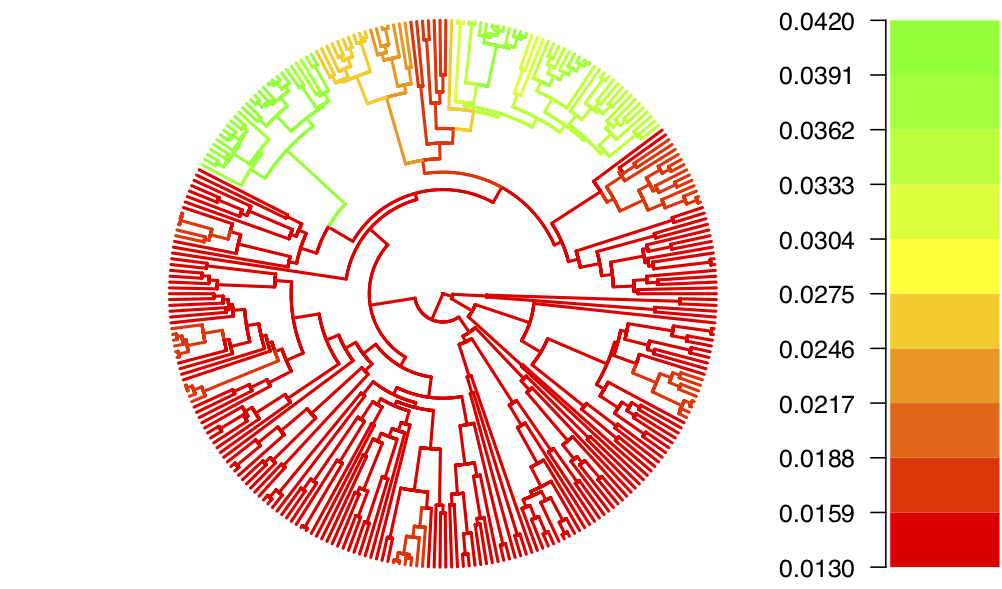
We can see that while most of the tree shares one evolutionary regime (in red), some clades are inferred to have evolved under a second regime (in green), with higher birth and death rates. From this figure it is not possible to tell whether the clades coloured in yellow-orange represent a third intermediate regime, or whether there is uncertainty as to which of the two regimes they belong to.
Going back to the rates log file and using the full posterior distribution rather than just the median, we see that the intermediate colour is likely due to uncertainty rather than a third regime.
Useful Links
- Bayesian Evolutionary Analysis with BEAST 2 (Drummond & Bouckaert, 2014)
- BEAST 2 website and documentation: http://www.beast2.org/
- BEAST 1 website and documentation: http://beast.bio.ed.ac.uk
- Join the BEAST user discussion: http://groups.google.com/group/beast-users
Relevant References
- Barido-Sottani, J., Vaughan, T. G., & Stadler, T. (2020). A Multi-Type Birth-Death model for Bayesian inference of lineage-specific birth and death rates. Systematic Biology. https://doi.org/10.1093/sysbio/syaa016
- Bouckaert, R., Heled, J., Kühnert, D., Vaughan, T., Wu, C.-H., Xie, D., Suchard, M. A., Rambaut, A., & Drummond, A. J. (2014). BEAST 2: a software platform for Bayesian evolutionary analysis. PLoS Computational Biology, 10(4), e1003537. https://doi.org/10.1371/journal.pcbi.1003537
- McGuire, J. A., Witt, C. C., Remsen, J. V., Corl, A., Rabosky, D. L., Altshuler, D. L., & Dudley, R. (2014). Molecular Phylogenetics and the Diversification of Hummingbirds. Current Biology, 24(8), 910–916. https://doi.org/10.1016/j.cub.2014.03.016
- Drummond, A. J., & Bouckaert, R. R. (2014). Bayesian evolutionary analysis with BEAST 2. Cambridge University Press.
Citation
If you found Taming the BEAST helpful in designing your research, please cite the following paper:
Joëlle Barido-Sottani, Veronika Bošková, Louis du Plessis, Denise Kühnert, Carsten Magnus, Venelin Mitov, Nicola F. Müller, Jūlija Pečerska, David A. Rasmussen, Chi Zhang, Alexei J. Drummond, Tracy A. Heath, Oliver G. Pybus, Timothy G. Vaughan, Tanja Stadler (2018). Taming the BEAST – A community teaching material resource for BEAST 2. Systematic Biology, 67(1), 170–-174. doi: 10.1093/sysbio/syx060