


Background
Before diving into performing complex analyses with BEAST2 one needs to understand the basic workflow and concepts. While BEAST2 tries to be as user-friendly as possible, the amount of possibilities can be overwhelming.
In this simple tutorial you will get acquainted with the basic workflow of BEAST2 and the software tools most commonly used to interpret the results of analyses. Bear in mind that this tutorial is designed only to help you get started using BEAST2. This tutorial does not discuss all the choices and concepts in detail, as they are discussed in further tutorials. Interspersed throughout the tutorial are topics for discussion. These discussion topics are optional, however if you work through them you will have a better understanding of the concepts discussed in this tutorial. Feel free to skip the discussion topics and come back to them later, while running the analysis file, or after finishing the whole tutorial.
Programs used in this Exercise
BEAST2 - Bayesian Evolutionary Analysis Sampling Trees 2
BEAST2 (http://www.beast2.org) is a free software package for Bayesian evolutionary analysis of molecular sequences using MCMC and strictly oriented toward inference using rooted, time-measured phylogenetic trees. This tutorial is written for BEAST v2.7.x (Bouckaert et al., 2014; Bouckaert et al., 2019).
BEAUti2 - Bayesian Evolutionary Analysis Utility
BEAUti2 is a graphical user interface tool for generating BEAST2 XML configuration files.
Both BEAST2 and BEAUti2 are Java programs, which means that the exact same code runs on all platforms. For us it simply means that the interface will be the same on all platforms. The screenshots used in this tutorial are taken on a Mac OS X computer; however, both programs will have the same layout and functionality on both Windows and Linux. BEAUti2 is provided as a part of the BEAST2 package so you do not need to install it separately.
TreeAnnotator
TreeAnnotator is used to produce a summary tree from the posterior sample of trees using one of the available algorithms. It can also be used to summarise and visualise the posterior estimates of other tree parameters (e.g. node height).
TreeAnnotator is provided as a part of the BEAST2 package so you do not need to install it separately.
Tracer
Tracer (http://beast.community/tracer) is used to summarise the posterior estimates of the various parameters sampled by the Markov Chain. This program can be used for visual inspection and to assess convergence. It helps to quickly view median estimates and 95% highest posterior density intervals of the parameters, and calculates the effective sample sizes (ESS) of parameters. It can also be used to investigate potential parameter correlations. We will be using Tracer v1.7.x.
FigTree
FigTree (http://beast.community/figtree) is a program for viewing trees and producing publication-quality figures. It can interpret the node-annotations created on the summary trees by TreeAnnotator, allowing the user to display node-based statistics (e.g. posterior probabilities). We will be using FigTree v1.4.x.
DensiTree
Bayesian analysis using BEAST2 provides an estimate of the uncertainty in tree space. This distribution is represented by a set of trees, which can be rather large and difficult to interpret. DensiTree is a program for qualitative analysis of sets of trees. DensiTree allows to quickly get an impression of properties of the tree set such as well-supported clades, distribution of tree heights and areas of topological uncertainty.
DensiTree is provided as a part of the BEAST2 package so you do not need to install it separately.
Practical: Running a simple analysis with BEAST2
This tutorial will guide you through the analysis of an alignment of sequences sampled from twelve primate species. The aim of this tutorial is to co-estimate the gene phylogeny and the rate of evolution. More generally, this tutorial aims to introduce new users to a basic workflow and point out the steps towards performing a full analysis of sequencing data within a Bayesian framework using BEAST2.
After completing this tutorial you should be able to:
- Set up all the components of a simple BEAST2 analysis in BEAUti2
- Use a calibration node to calibrate the molecular clock
- Use Tracer, FigTree and DensiTree to check convergence and analyse results
The Data
Before we can start, we need to download the input data for the tutorial. For this tutorial we use a single NEXUS file, primate-mtDNA.nex, which contains a sequence alignment and metadata of the twelve primate mitochondrial genomes we will be analysing. Among other information, the metadata contains information to partition the alignment into 4 regions:
- Non-coding region
- 1st codon positions
- 2nd codon positions
- 3rd codon positions
The alignment file can be downloaded from the Taming the BEAST website at https://taming-the-beast.org/tutorials/Introduction-to-BEAST2/ or from Github.
Downloading from taming-the-beast.org
A link to the alignment file,
primate-mtDNA.nex, is on the left-hand panel, under the heading Data. Right-click on the link and select “Save Link As…“ (Firefox and Chrome) or “Download Linked File As…“ (Safari) and save the file to a convenient location on your local drive. Note that some browsers will automatically change the extension of the file from.nexto.nex.txt. If this is the case, simply rename the file again.Alternatively, if you left-click on the link most browsers will display the alignment file. You can then press File > Save As to store a local copy of the file. Note that some browsers will inject an HTML header into the file, which will make it unusable in BEAST2 (making this the less preferable option for downloading data files).
In the same way you can also download example
.xmlfiles for the analyses in this tutorial, as well as pre-cooked output.logand.treesfiles. We recommend only downloading these files to check your results or if you become seriously stuck.
Downloading from Github
If you navigate to the Github repository you can either download the raw data files directly from Github or clone/download the repository to your local drive.
Note that this tutorial is distributed under a CC BY 4.0 license, which gives anyone the right to freely use (and modify) it, as long as appropriate credit is given and the updated material is licensed in the same fashion.
Creating the Analysis File with BEAUti
To run analyses with BEAST, one needs to prepare a configuration file in XML format that contains everything BEAST2 needs to run an analysis. A BEAST2 XML file contains:
- The data (typically a sequence alignment)
- The model specification
- Initial values and parameter constraints
- Settings of the MCMC algorithm
- Output options
Even though it is possible to create such files from scratch in a text editor, it can be complicated and is not exactly straightforward. BEAUti is a user-friendly program designed to aid you in producing a valid configuration file for BEAST. If necessary, that file can later be edited by hand, but it is recommended to use BEAUti for generating the files (at least for the initial round of analysis).
Begin by starting BEAUti2.
Importing the alignment
To give BEAST2 access to the data, the alignment has to be added to the configuration file.
Drag and drop the file
primate-mtDNA.nexinto the open BEAUti window (it should be on the Partitions tab).Alternatively, use File > Import Alignment or click on the + in the bottom left-hand corner of the window, then locate and click on the alignment file.
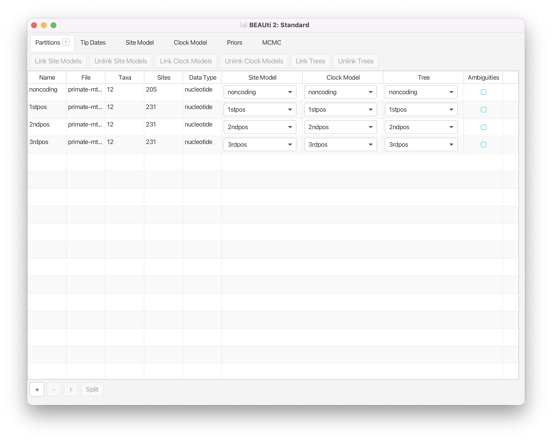
Once you have done that, the data should appear in the BEAUti window which should look as shown in Figure 1.
Setting up shared models
A common way to account for site-to-site rate heterogeneity (variation in substitution rates between different sites) is to use a Gamma site model. In this model, one assumes that rate variation follows a Gamma distribution. To make the analysis tractable the Gamma distribution is discretised to a small number of bins (4-6 usually). The mean of each bin then acts as a multiplier for the overall substitution rate. The transition probabilities are then calculated for each scaled substitution rate. To calculate the likelihood for a site, P(data | tree, substitution model) is calculated under each Gamma rate category and the results are summed up to average over all possible rates. This is a handy approach if one suspects that some sites are mutating faster than others but the precise position of these sites in the alignment is unknown or random.
Another way to account for site-to-site rate heterogeneity is to split the alignment into explicit partitions, and specify an independent substitution model for each partition. This is especially relevant when one knows exactly which positions in the alignment are expected to evolve at different rates. In our example, we split the alignment into coding and non-coding regions, and further split the coding region into 1st, 2nd and 3rd codon positions. This information is encoded as metadata into the .nex file, which BEAUti automatically processes to produce the four partitions in the Partitions tab as shown in Figure 1.
Double-click on the different partitions (under the File column) to view the individual alignments.
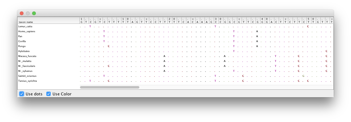
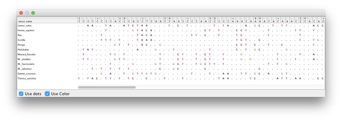
By looking at the alignments for the 2nd and 3rd codon positions (Figure 2 and Figure 3) we can immediately see a clear difference between the two codon positions. For the 2nd codon position many of the ancestral relationships are clear from shared substitutions between groups, for instance between the great apes (Homo sapiens, Pan, Gorilla and Pongo - humans, chimpanzees, gorillas and orangutans) and between the old-world monkeys (Macaca fuscata, M. mulatta, M. fascicularis and M. sylvanus - the macaques). The lesser apes (represented by Hylobates - gibbons) share most substitutions with the great apes, but occasionally share a substitution with the macaques. For the 3rd codon position there are many more substitutions and the groupings are not as clear.
Topic for discussion: Do you think there is a good case for using independent substitution models on the different partitions in the
.nexfile? Do you think this is sufficient for taking all site-to-site rate variation into account?How would you account for rate variation between sites within each partition?
Since all of the sequences in this dataset are from the mitochondrial genome (which is not believed to undergo recombination in birds and mammals) they all share the same ancestry. By default, BEAST2 would recover a separate, independent time-calibrated tree for each partition, so we need to make sure that it uses all data to recover only a single shared tree. For the sake of simplicity, we will also assume that the partitions have the same evolutionary branch-rate distribution, and hence share the clock model as well.
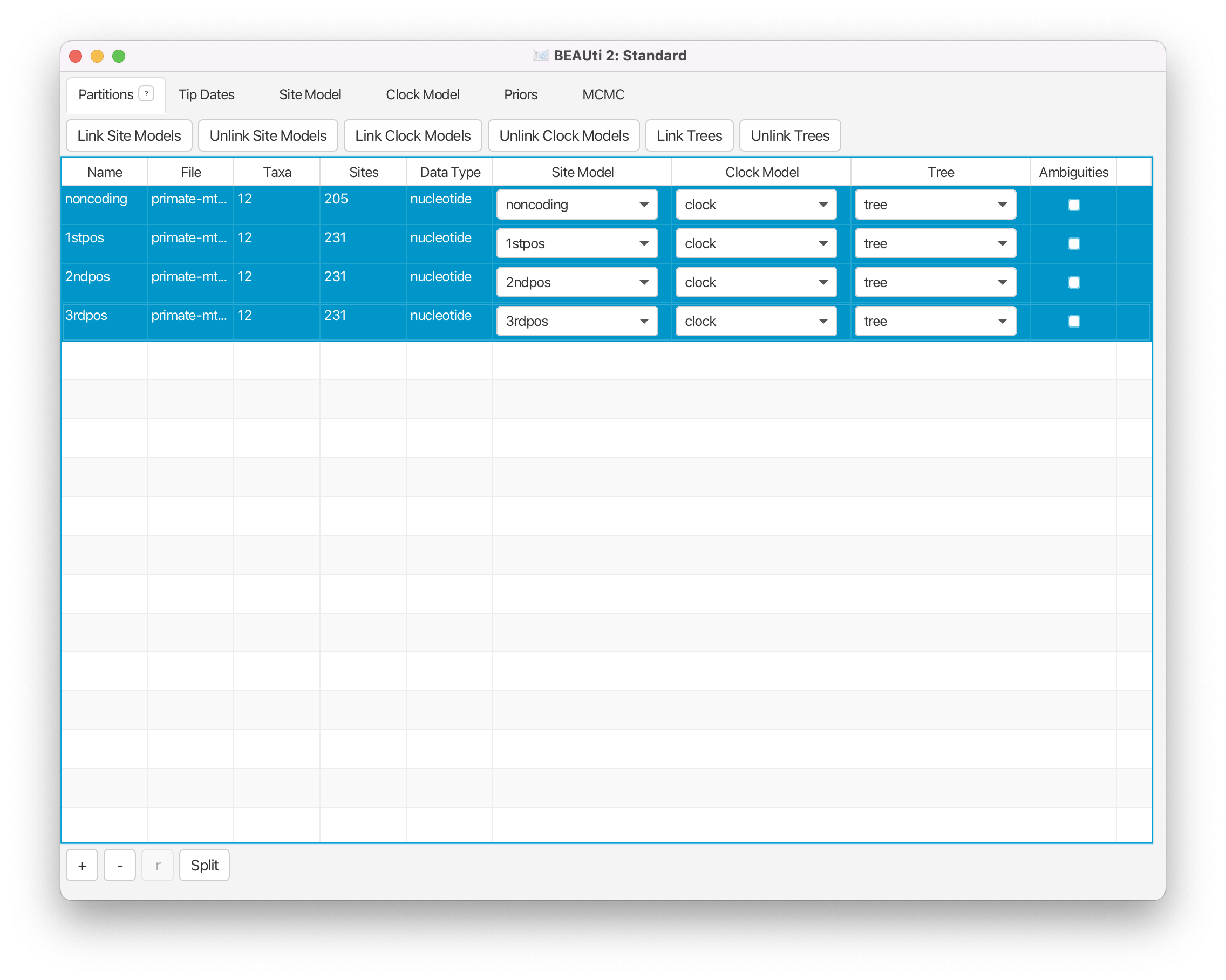
To make sure that the partitions share the same evolutionary history we need to link the clock model and the tree in BEAUti.
Select all four data partitions the Partitions panel (use shift+click) and click the Link Trees and Link Clock Models buttons.
You will see that the Clock Model and the Tree columns in the table both changed to say noncoding. Now we will rename both models such that the following options and generated log files are easier to read. The resulting setup should look as shown in Figure 4.
Click on the first drop-down menu in the Clock Model column and rename the shared clock model to
clock.Likewise, rename the shared tree to
tree.
Setting the substitution model
In this analysis all of our sequences come from extant species and were thus all sampled in the present day (assumed to be ). Therefore we do not need to set sampling dates and we skip the Tip Dates panel. Next, we need to set the substitution model in the Site Model tab.
Select the Site Model tab.
The options available in this panel depend on whether the alignment data are in nucleotides, amino-acids, binary data or general data. The settings available after loading the alignment will contain the default values we normally want to modify.
The panel on the left shows each partition. Remember that we did not link the substitution models in the previous step for the different partitions, so each partition evolves under a different substitution model, i.e. we assume that different positions in the alignment accumulate substitutions differently. We will need to set the site model separately for each part of the alignment as these models are unlinked. However, we think that all partitions evolve according to the same general model (albeit with different parameter values).
Make sure that
noncodingis selected.
- Check the estimate checkbox for Substitution Rate.
- Set the Gamma Category Count to 4.
- Check the estimate box for the Shape parameter (it should already be checked).
- Select HKY in the Subst Model drop-down menu.
- Ensure that the estimate box for Kappa is checked (it should already be checked).
- Select Empirical from the Frequencies drop-down menu.
Note that when you checked estimate for the substitution rate the greyed out Fix mean substitution rate box at the bottom of the window was also automatically checked.
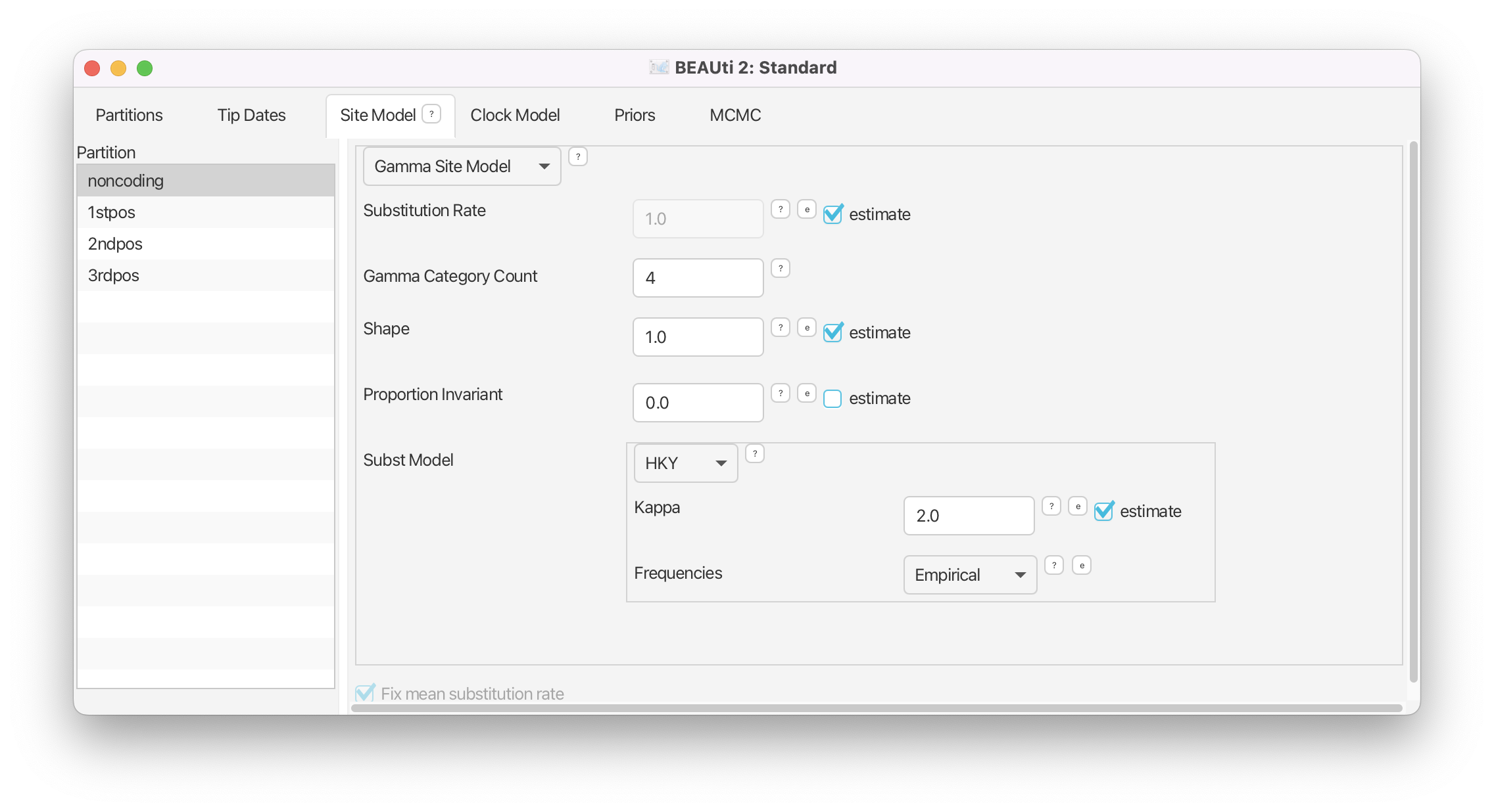
The panel should now look like Figure 5.
We are using an HKY substitution model with empirical frequencies. This will fix the frequencies to the proportions observed in the partition. This approach means that we can get a good fit to the data without explicitly estimating these parameters. To model site-to-site rate variation within each partition we use a discrete Gamma site model with 4 categories. Now we could repeat the above steps for each of the remaining partitions or we can take a shortcut.
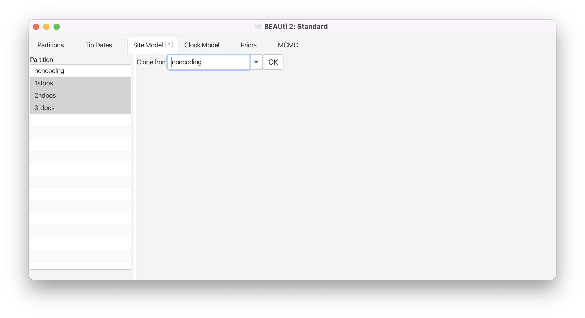
Select the remaining three partitions (use shift+click). The window will now look like Figure 6.
Select
noncodingand click OK to to clone the site model for the other three partitions fromnoncoding.
Topic for discussion: Can you figure out the reason why Fix mean substitution rate was automatically checked when you checked estimate for the substitution rate? Don’t worry if you can’t figure it out, it is explained in detail in later tutorials.
Setting the clock model
Next, select the Clock Model tab at the top of the main window. This is where we set up the molecular clock model. For this exercise we are going to leave the selection at the default value of a strict molecular clock, because this data is very clock-like and does not need rate variation among branches to be included in the model.
Click on the Clock Models tab and view the setup (but don’t do anything).
Note that the estimate box next to Mean clock rate is not checked.
Setting priors
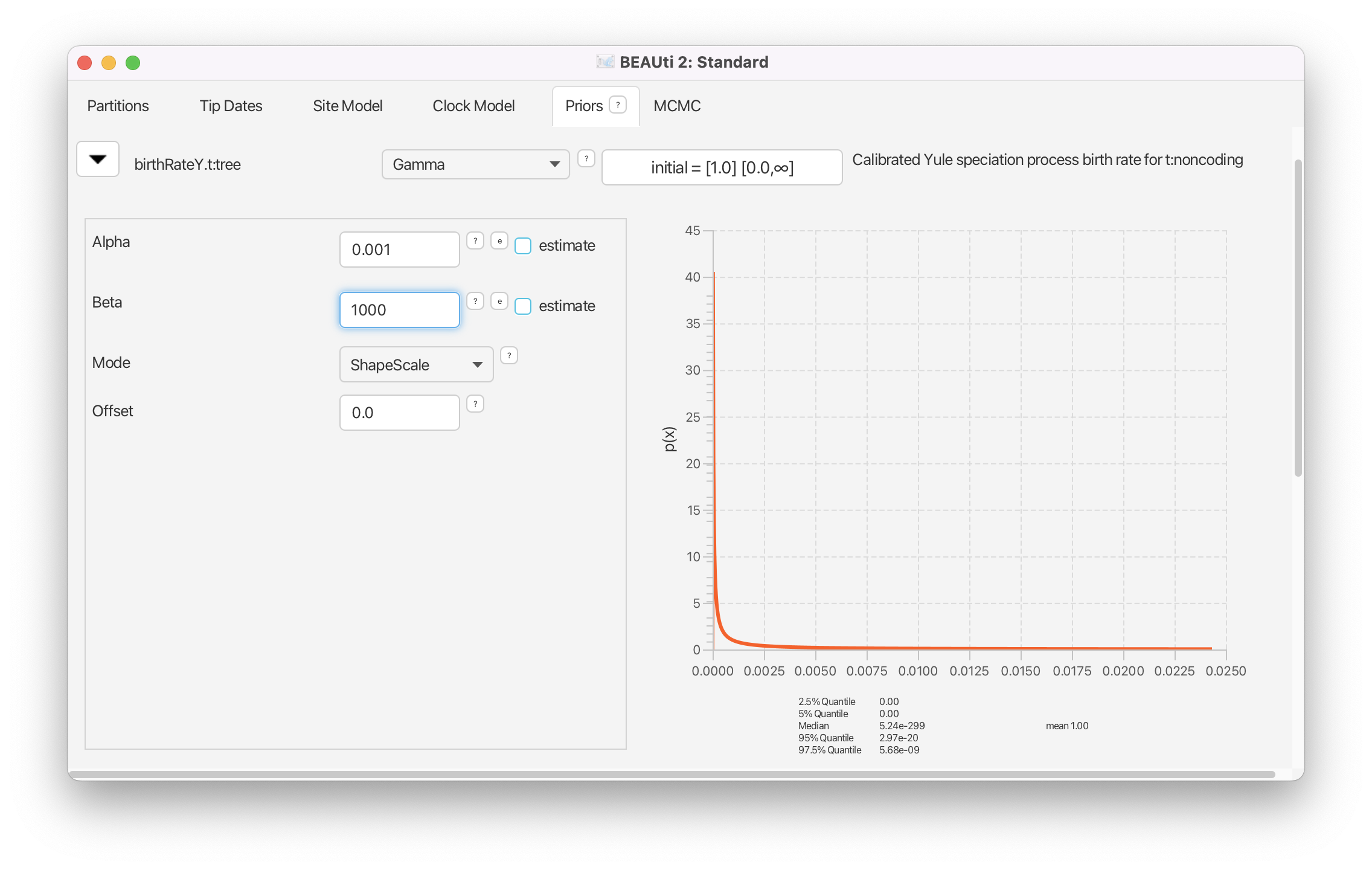
The Priors tab allows prior distributions to be specified for each model parameter. The model selections made in the Site Model and Clock Model tabs determine which parameters are included in the model. For each of these parameters a prior distribution needs to be specified. It is also possible to specify hyperpriors (and hyper-hyperpriors etc.) for each of the model parameters. We also need to specify a prior for the Tree. In this example the tree prior is a null model for species diversity over time within the primates.
Here we specify that we wish to use the Calibrated Yule model as the tree prior. This is a simple model of speciation that is generally appropriate when considering sequences from different species.
Go to the Priors tab and select Calibrated Yule Model in the drop-down menu next to Tree.t:tree.
The birthRate parameter measures the rate of speciation in the calibrated Yule model. We will set an unspecific Gamma prior for this parameter.
For birthRateY.t:tree select Gamma from the drop-down menu
- Expand the options for birthRateY.t:tree using the arrow button on the left.
- Set the Alpha (shape) parameter to 0.001 and the Beta (scale) parameter to 1000.
Note that BEAUti displays a plot of the prior distribution on the right, as well as a few of its quantiles. This is for easy reference and can help us to decide if a prior is appropriate. The unspecific Gamma prior we are using is defined on and has a very broad range of values included between its 2.5% and 97.5% quantiles.
If we wanted to add a hyperprior on one of the parameters of the Gamma prior we would check the estimate box on the right of the parameter. We could also change the initial values or limits of the model parameters by clicking on the boxes next to the drop-down menus. Do not do this here, as we are not adding any hyperpriors or changing limits in this analysis!
We will leave the rest of the priors on their default values! The BEAUti panel should look as shown in Figure 7.
Please note that in general using default priors is frowned upon as priors are meant to convey your prior knowledge of the parameters. It is important to know what information the priors add to the MCMC analysis and whether this fits your particular situation. In our case the default priors are suitable for this particular analysis, however for further, more complex analyses, we will require a clear idea of what the priors mean. Getting this understanding is difficult and comes with experience. The topic of choosing priors is discussed in more detail in later tutorials.
Adding a calibration node
Since all of the samples come from a single time point, there is no information on the actual height of the phylogenetic tree in time units. That means the tree height (tMRCA) and substitution rate parameters will not be distinguishable and BEAST2 will only be able to estimate their product. To allow BEAST2 to separate these two parameters we need to input additional information that will help calibrate the tree in time.
In a Bayesian analysis, additional information from external sources should be encoded in the form of a prior distribution. Thus, we will have to add a new prior to the model.
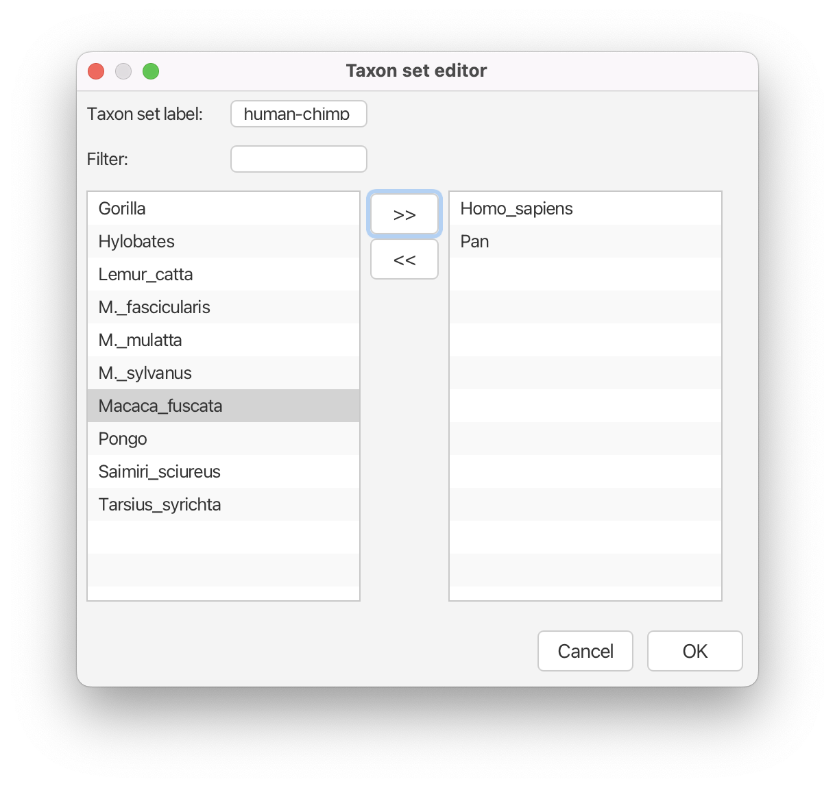
To add an extra prior to the model, press the + Add Prior button below the list of priors. If this doesn’t automatically open a Taxon set editor window, select MRCA Prior from the drop-down menu.
You will see a dialogue box (Taxon set editor) that allows you to select a subset of taxa from the phylogenetic tree. Once you have created a taxon set you will be able to add calibration information for its most recent common ancestor (MRCA) later on.
- Set the Taxon set label to
human-chimp.- Locate
Homo_sapiensin the left hand side list and click the » button to add it to thehuman-chimptaxon set.- Locate
Panin the left hand side list and click the » button to add it to thehuman-chimptaxon set.
The taxon set should now look like Figure 8.
Click the OK button to add the newly defined taxon set to the prior list.
The new node we have added is a calibrated node on the human-chimpanzee split to be used in conjunction with the Calibrated Yule prior. In order for that to work we need to enforce monophyly. This will constrain the tree topology so that the human-chimp grouping is kept monophyletic during the course of the MCMC analysis.
Check the monophyletic checkbox next to the human-chimp.prior.
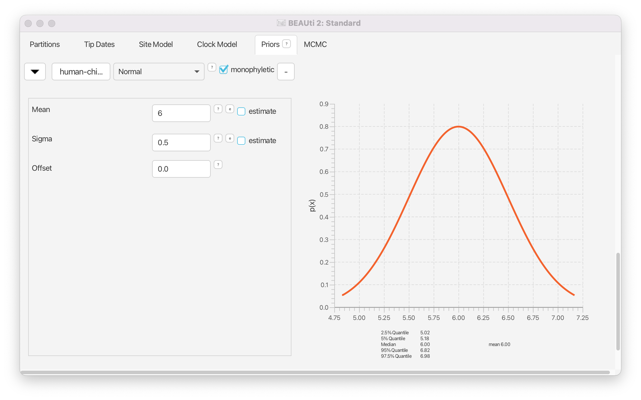
We now need to specify a prior distribution on the calibration node based on our prior knowledge from fossils in order to calibrate our tree. We will use a Normal distribution with mean 6 MYA and a standard deviation of 0.5 million years. This will give a central 95% range of about 5-7 million years, which roughly corresponds to the current consensus estimate of the date of the most recent common ancestor of humans and chimpanzees.
Select Normal from the drop-down menu to the right of the newly added human-chimp.prior.
- Expand the distribution options using the arrow button on the left.
- Set the Mean of the distribution to 6.
- Set the Sigma of the distribution to 0.5.
The final setup of the calibration node prior should look as shown in Figure 9.
Topic for discussion: After setting the calibration node prior a new prior for
clockrate.c:clockmagically appeared in the priors tab! If you go back to the Clock model tab you’ll see that the estimate box next to Mean clock rate is now checked and greyed out (cannot be unchecked).What just happened?
Setting the MCMC options
Finally, the MCMC tab allows us to control the length of the MCMC chain and the frequency of stored samples. It also allows one to change the output file names.
Go to the MCMC tab.
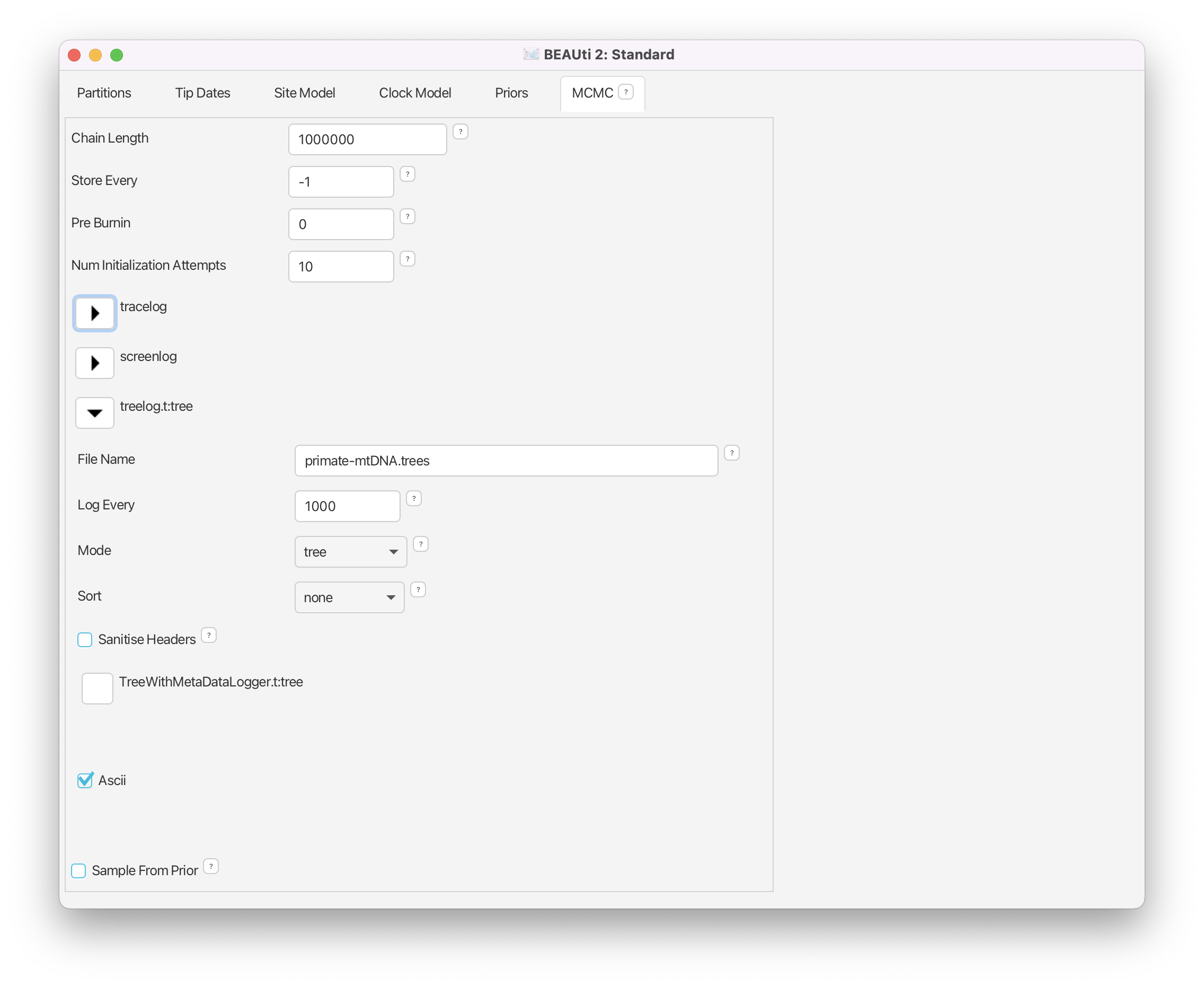
The Chain Length parameter specifies the number of steps the MCMC chain will make before finishing (i.e. the number of accepted proposals). This number depends on the size of the dataset, the complexity of the model and the precision of the answer required. The default value of 10’000’000 is arbitrary and should be adjusted accordingly. For this small dataset we initially set the chain length to 1’000’000 such that this analysis will take only a few minutes on most modern computers (rather than hours). We leave the Store Every and Pre Burnin fields at their default values.
Set the Chain Length to 1’000’000.
Below these general settings you will find the logging settings. Each particular option can be viewed in detail by clicking the arrow to the left of it. You can control the names of the log files and how often values will be stored in each of the files.
Start by expanding the tracelog options. This is the log file you will use later to analyse and summarise the results of the run. The Log Every parameter for the log file should be set relative to the total length of the chain. Sampling too often will result in very large files with little extra benefit in terms of the accuracy of the analysis. Sampling too sparsely will mean that the log file will not record sufficient information about the distributions of the parameters. We normally want to aim to store no more than 10’000 samples so this should be set to no less than chain length/10’000. For this analysis we will make BEAST2 write to the log file every 200 samples.
Expand the tracelog options.
- Set the Log Every parameter to 200.
- Leave the filename as is (
$(filebase).log).
Next, expand the screenlog options. The screen output is simply for monitoring the program’s progress. Since it is not so important, especially if you run your analysis on a remote computer or a computer cluster, the Log Every can be set to any value. However, if it is set too small, the sheer quantity of information being displayed on the screen will actually slow the program down. For this analysis we will make BEAST2 log to screen every 1’000 samples, which is the default setting.
Expand the screenlog options.
- Leave the Log Every parameter at the default value of 1’000.
Finally, we can also change the tree logging frequency by expanding treelog.t:tree. For big trees with many taxa each individual tree will already be quite large, thus if you log lots of trees the tree files can easily become extremely large. You will be amazed at how quickly BEAST can fill up even the biggest of drives if the tree logging frequency is too high! For this reason it is often a good idea to set the tree logging frequency lower than the trace log (especially for analyses with many taxa). However, be careful, as the post-processing steps of some models (such as the Bayesian skyline plot) require the trace and tree logging frequencies to be identical!
Expand the treelog.t:tree options.
- Set the File Name to
primate-mtDNA.trees.- Leave the Log Every parameter at the default value of 1’000.
The final setup should look as in Figure 10.
Generating the XML file
We are now ready to create the BEAST2 XML file. This is the final configuration file BEAST2 can use to execute the analysis.
Save the XML file under the name
primates-mtDNA.xmlusing File > Save.
Running the analysis
Now run BEAST2 and provide your newly created XML file as input. You can also change the random number seed for the run. This number is the starting point of a pseudo-random number chain BEAST2 will use to generate the samples. As computers are unable to generate truly random numbers, we have to resort to generating deterministic sequences of numbers that only look random, but will be identical when the starting seed is the same. If your MCMC run converges to the true posterior then you will be able to draw the same conclusions regardless of which random seed is provided. However, if you want to exactly reproduce the results of a run you need to start it with the same random number seed.
Run the BEAST2 program.
- Select
primates-mtDNA.xmlas the Beast XML File.- Set the Random number seed to 777 (or pick your favourite number).
- Check the Use BEAGLE library if available checkbox. If you have previously installed BEAGLE this will make the analysis run faster.
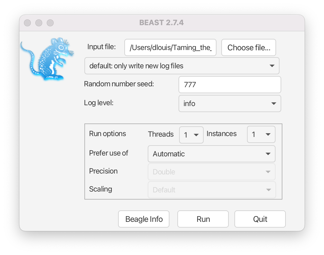
The BEAST2 window should look similar to Figure 11.
Run BEAST2 by clicking the
Runbutton.
BEAST2 will run until the specified number of steps in the chain is reached. While it is running, it will print the screenlog values to a console and store the tracelog and tree log values to files located in the same folder as the configuration XML file. The screen output will look approximately as shown in Figure 12.
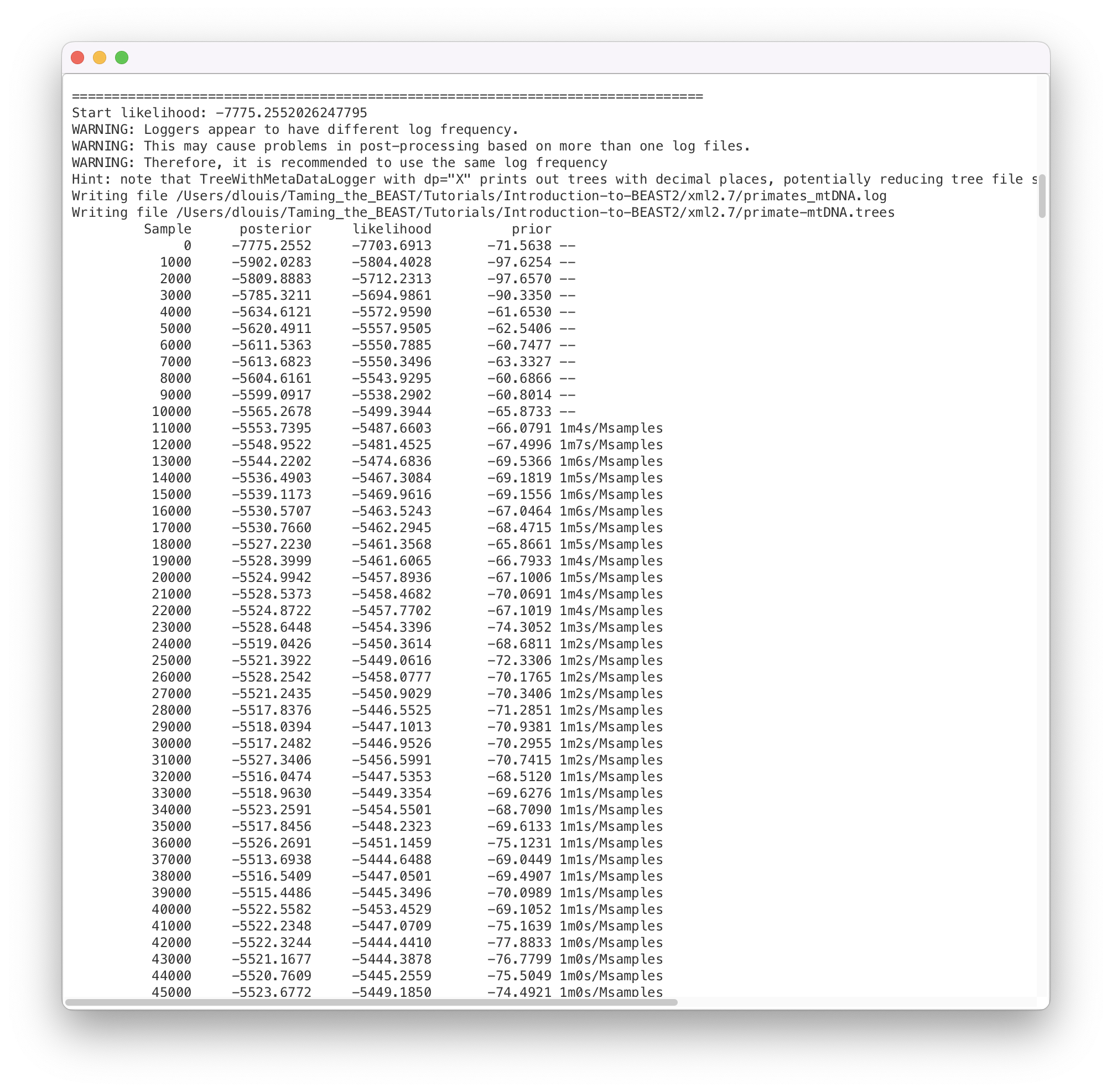
The window will remain open when BEAST2 finished running the analysis. When you try to close it, you may see BEAST2 asking the question: “Do you wish to save?”. Note that your log and trees files are always saved, no matter what answer you choose for this question. Thus, the question is only restricted to saving the BEAST2 screen output (which contains some information about the hardware configuration, initial values, operator acceptance rates and running time that are not stored in the other output files).
Topic for discussion: While the analysis is running see if you can identify which parts of the setup in BEAUti are concerned with the data, the model and the MCMC algorithm.
Open the XML file in your favourite text editor. Can you recognize any of the values you set in BEAUti? Can you identify the data, model specification and MCMC settings in the XML file?
Can you find the likelihood, priors and hyperpriors in the XML file?
Analysing the results
Once BEAST2 has finished running, open Tracer to get an overview of BEAST2 output. When the main window has opened, choose File > Import Trace File... and select the file called primate-mtDNA.log that BEAST2 has created, or simply drag the file from the file manager window into Tracer.
Open Tracer. Drag and drop the
primate-mtDNA.logfile that BEAST2 created into the open Tracer window.Alternatively, use File > Import Trace File… (or press the + button below the Trace Files panel) then locate and click on
primate-mtDNA.log.
The Tracer window should look as shown in Figure 13.
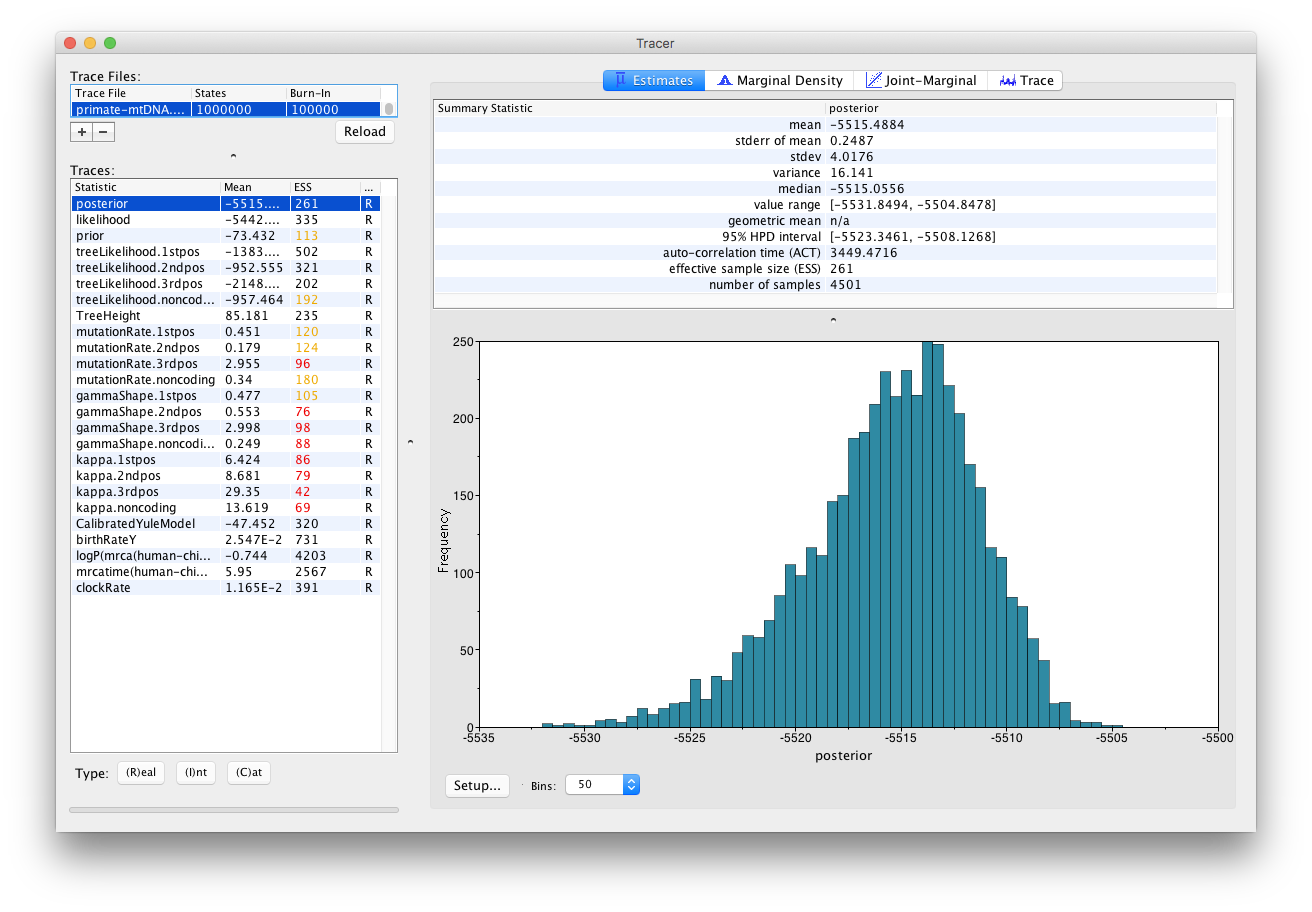
Tracer provides a few useful summary statistics on the results of the analysis. On the left side in the top window it provides a list of log files loaded into the program at the moment. The window below shows the list of statistics logged in each file. For each statistic it gives a list of summary values such as the mean, standard error, median, and others it can compute from the data. The summary values are displayed in the top right window and a histogrom showing the distribution of the statistic is in the bottom right window.
The log file contains traces for the posterior (this is the natural logarithm of the product of the tree likelihood and the prior density), prior, the likelihood, tree likelihoods and other continuous parameters. Selecting a trace on the left brings up the summary statistics for this trace on the right hand side. When first opened, the posterior trace is selected and various statistics of this trace are shown under the Estimates tab.
For each loaded log file we can specify a Burn-In, which is shown in the file list table (top left) in Tracer. The burn-in is intended to give the Markov Chain time to reach its equilibrium distribution, particularly if it has started from a bad starting point. A bad starting point may lead to over-sampling regions of the posterior that actually have very low probability, before the chain settles into the equilibrium distribution. Burn-in allows us to simply discard the first N samples of a chain and not use them to compute the summary statistics. Determining the number of samples to discard is not a trivial problem and depends on the size of the dataset, the complexity of the model and the length of the chain. A good rule of thumb is to always throw out at least the first 10% of the whole chain length as the burn-in (however, in some cases it may be necessary to discard as much as 50% of the MCMC chain).
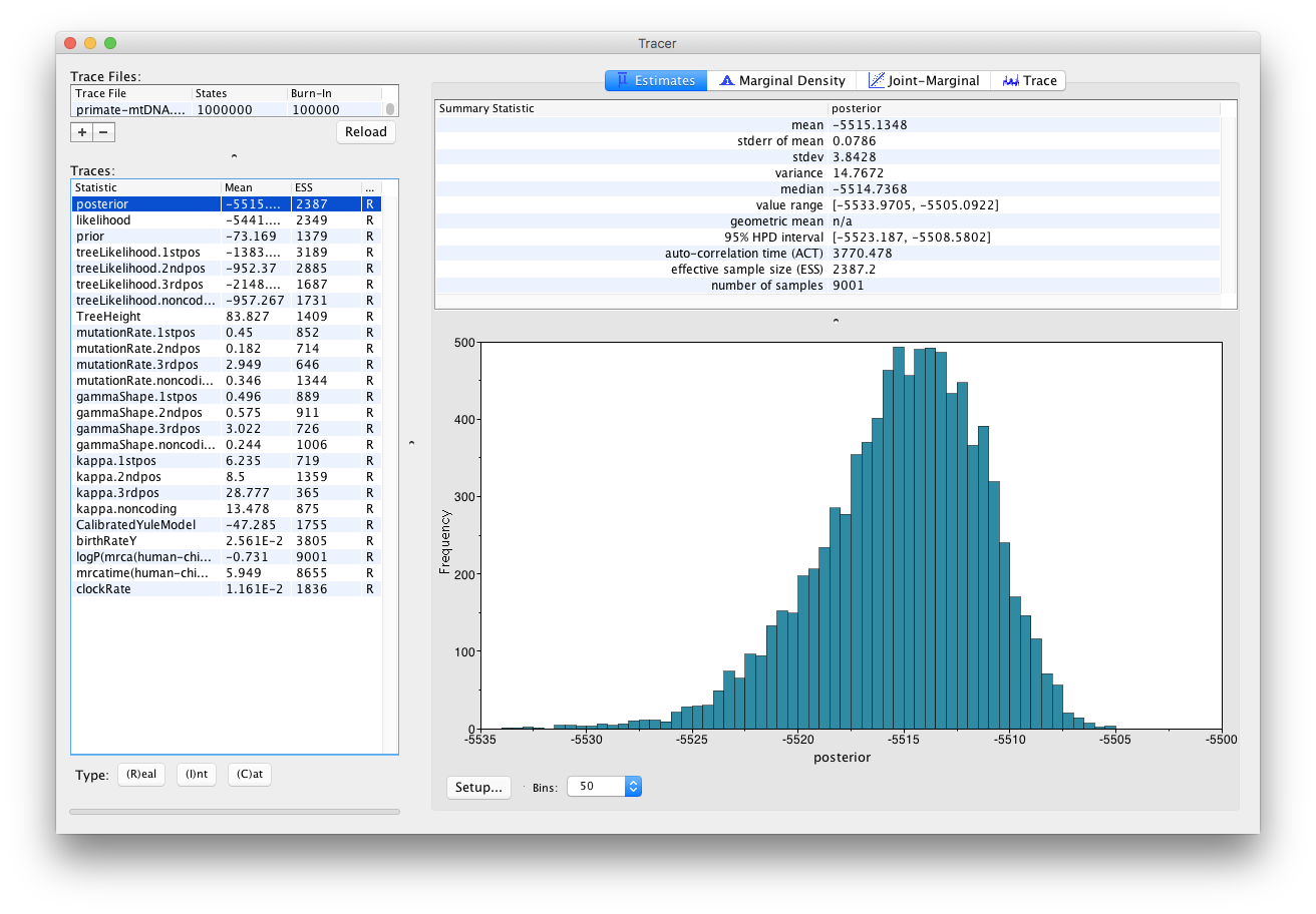
Select the TreeHeight statistic in the left hand list to look at the tree height estimated jointly for all partitions in the alignment. Tracer plots the (marginal posterior) histogram for the selected statistic and also give you summary statistics such as the mean and median. The 95% HPD stands for highest posterior density interval and represents the most compact interval on the selected statistic that contains 95% of the posterior density. It can be loosely thought of as a Bayesian analogue to a confidence interval. The TreeHeight statistic gives the marginal posterior distribution of the age of the root of the entire tree (that is, the tMRCA).
Select TreeHeight in the bottom left hand list in Tracer and view the different summary statistics on the right.
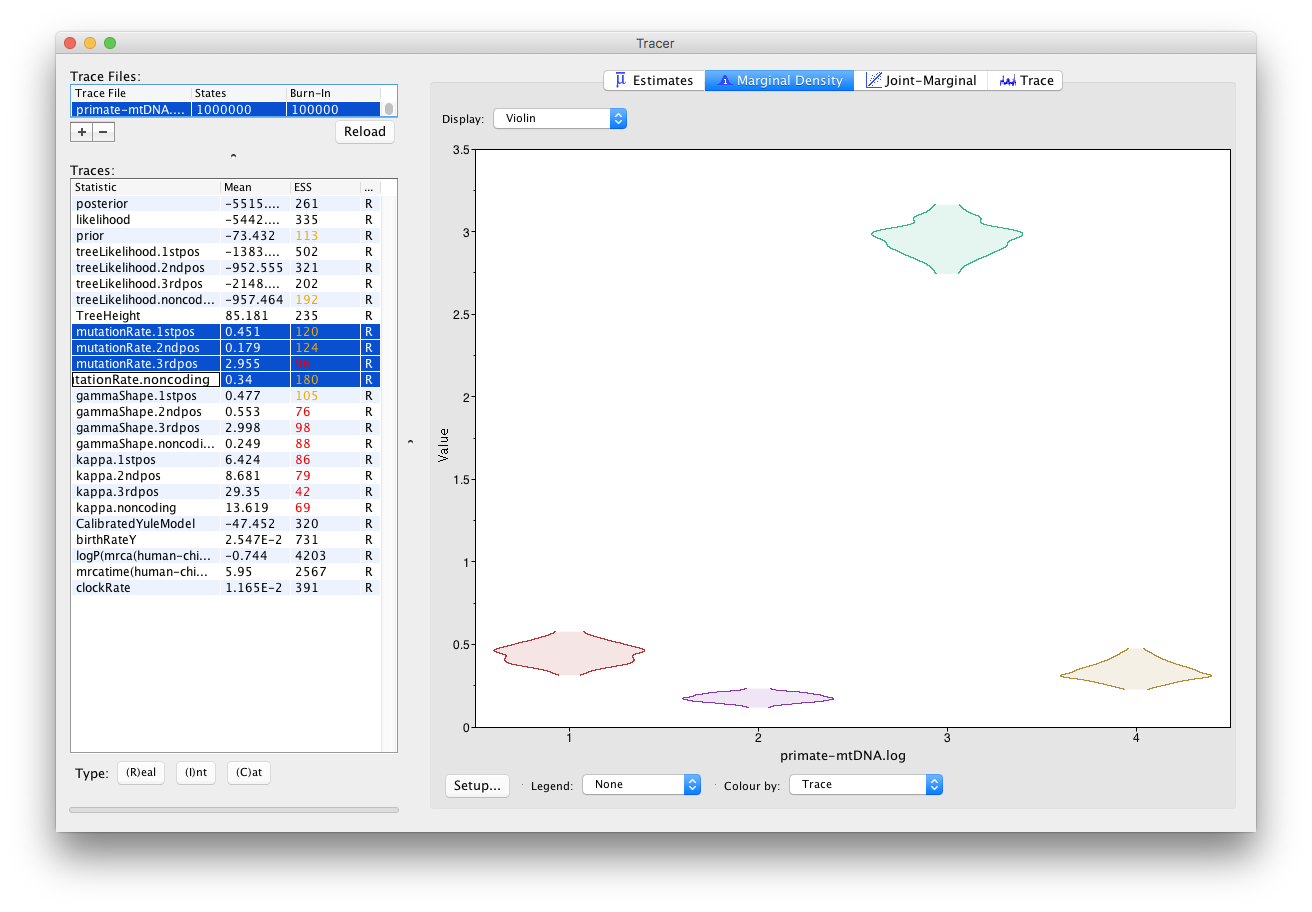
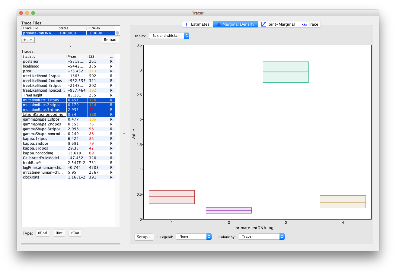
You can also compare estimates of different parameters in Tracer. Once a trace file is loaded into the program you can, for example, compare estimates of the different mutation rates corresponding to the different partitions in the alignment.
Select all four mutation rates by clicking the first mutation rate (mutationRate.noncoding), then holding Shift and clicking the last mutation rate (mutationRate.3rdpos).
Select the Marginal Density tab on the right to view the four distributions together.
Select different options in the Display drop-down menu to display the posterior distributions in different ways.
You will be able to see all four distributions in one plot, similar to what is shown in Figure 14.
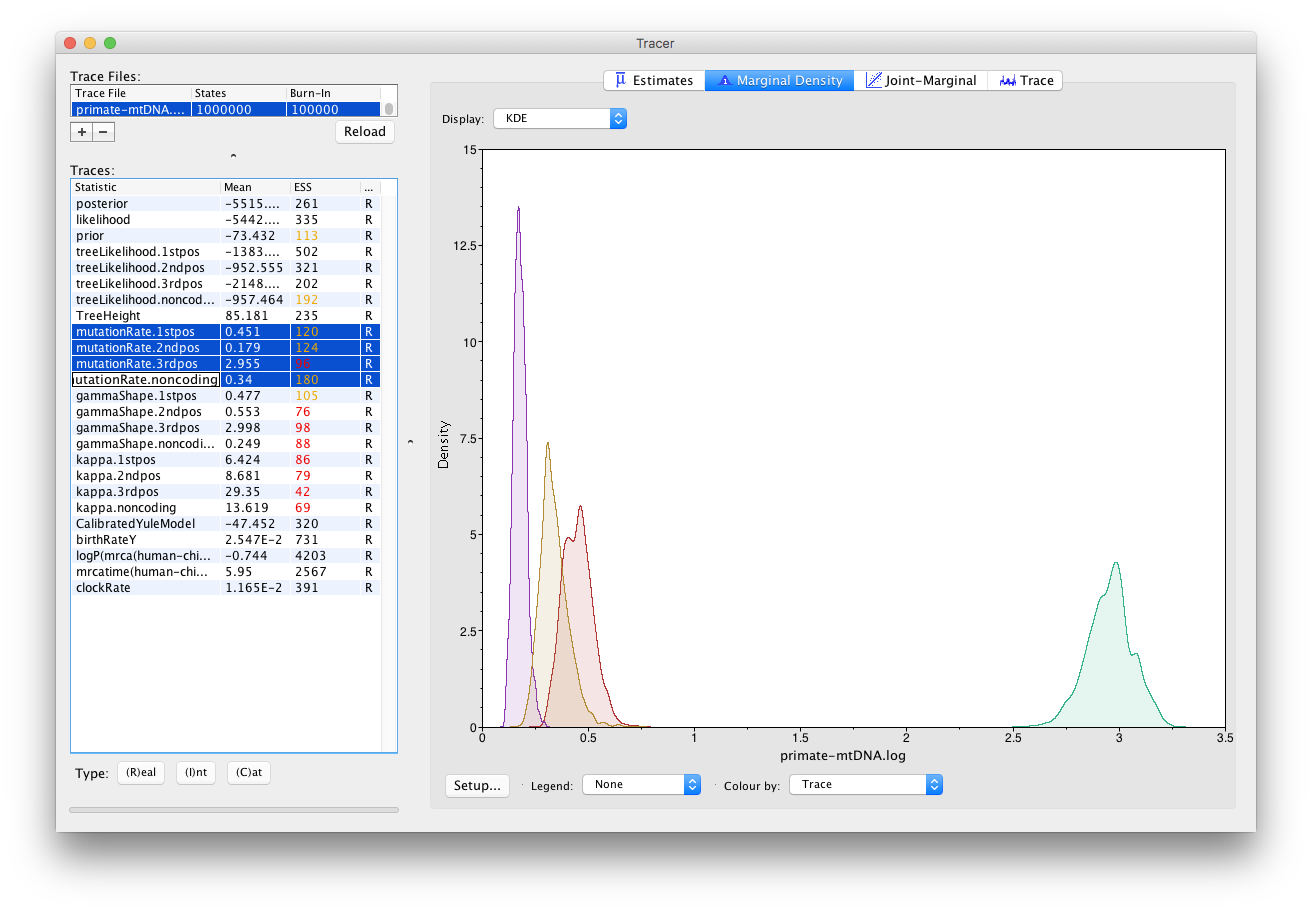
Topic for discussion: What can you deduce from the marginal densities of the 4 mutation rates? Does this make biological sense?
Why do you think the mutation rate of non-coding DNA is similar to the rates of 1st and 2nd codon positions? (display the legend on the plot to help with your analysis).
Analysing the posterior estimate quality
Two very important summary statistics that we should pay attention to are the Auto-Correlation Time (ACT) and the Effective Sample Size (ESS). ACT is the average number of states in the MCMC chain that two samples have to be separated by for them to be uncorrelated, i.e. for them to be independent samples from the posterior. The ACT is estimated from the samples in the trace (excluding the burn-in). The ESS is the number of independent samples that the trace is equivalent to. This is calculated as the chain length (excluding the burn-in) divided by the ACT.
The ESS is in general regarded as a quality-measure of the resulting sample sequence. It is unclear how to determine exactly how large should the ESS be for an analysis to be trustworthy. In general, an ESS of 200 is considered high enough to make the analysis useful. However, this is an arbitrary number and you should always use your own judgment to decide if the analysis has converged or not. As you can see in Figure 13, ESS values below 100 are coloured in red, which means that we should not trust the value of the statistics, and ESS values between 100 and 200 are coloured in yellow.
If a lot of statistics have red or yellow coloured ESS values, we have not sufficiently explored the posterior space. This is most likely a result of the chain not running long enough. Try running the same analysis as before, but with a longer chain.
First load the XML configuration file into BEAUti again by pressing File > Load and select the
primate-mtDNA.xmlfile. Within BEAUti, change the MCMC chain length parameter to 10’000’000 and change the tracelog frequency to 1’000.Change the trace and tree log file names in order to not overwrite the results of the previous analysis. You may add something like
_longbehind the name of the file, to obtainprimate-mtDNA_long.logfor the log file andprimate-mtDNA_long.treesfor trees file.Run BEAST2 again with the updated configuration file and the same seed of 777.
This will take a bit more time. Figure 15 shows the estimates from a longer run. In this case all parameters have ESS values larger than 200. Remember that MCMC is a stochastic algorithm, so if you set a different seed the actual numbers will not be exactly the same as those depicted in the figure.
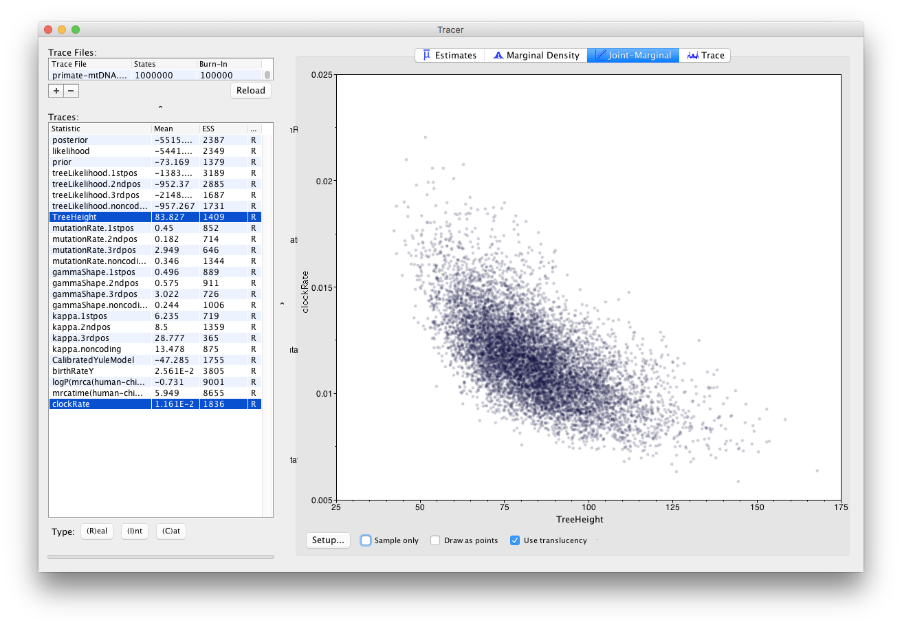
Tracer also allows us to look for correlations between parameters under the Joint Marginal tab, as shown in Figure 16. When two parameters are highly correlated this can lead to poor convergence of the MCMC chain (more on this in later tutorials).
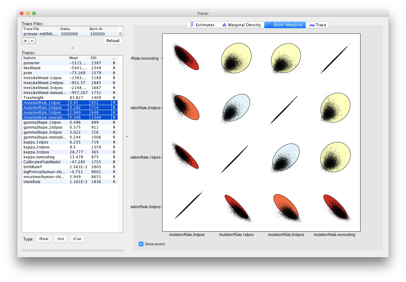
We can also look at correlations between more than two parameters.
Select all 4 mutation rates again
- Navigate to the Joint Marginal tab
- Check Show points
The panel should like Figure 17. The ellipses represent the covariance between pairs of parameters and make it easy to identify which pairs are correlated or anti-correlated. Is there a strong correlation or anti-correlation between some of our mutation rate parameters?
Topic for discussion: We have not explored the Trace tab in Tracer at all!
The Trace tab is primarily a diagnostic tool for checking convergence to the posterior, assessing the length of the burn-in and whether or not the chain is mixing well. There is a good argument to be made for this being the most important tab in the Tracer program and that it is the first tab users should look at.
Have a look at the individual parameter traces in the Trace tab, in both the short and long log files. Can you figure out why ESS values for some parameters are higher than others?
Do you think a burn-in of 10% is sufficient for this analysis?
Analysing tree estimates
In addition to generating a sample of parameter estimates, BEAST2 also produces a posterior sample of phylogenetic time-trees. It’s important to verify that these trees have also converged. However, this is a complex topic that requires a more detailed explanation. To keep things concise, we will skip it here. For more information, please refer to the Tree ESS Tutorial.
The trees we obtained from the analysis need to be summarised too before any conclusions about the quality of the posterior estimate can be made. One way to summarise them is by using the program TreeAnnotator. Until recently the maximum clade credibility tree (MCC) has been the default summary method in TreeAnotator. To produce MCC trees TreeAnotator takes the set of trees and find the best supported tree by maximising the product of the posterior clade probabilities. It will then annotate this representative summary tree with the mean ages of all the nodes and the corresponding 95% HPD ranges as well as the posterior clade probability for each node. A new point estimate, called a conditional clade distribution tree (CCD) has been proposed (Berling et al., 2025). It has been shown to outperform MCC in terms of accuracy (based on Robinson-Foulds distance to the true tree) and precision (how different are the point estimates calculated for replicate MCMC chains). CCD methods may produce a tree that would be well supported but has not been sampled during MCMC. This is beneficial for large trees and complex parameter regimes. Since both methods are still widely used, we show how to use them to summarise the posterior tree distribution. To save time, you may run just one method and compare it to the other using the example below.
Producing MCC tree
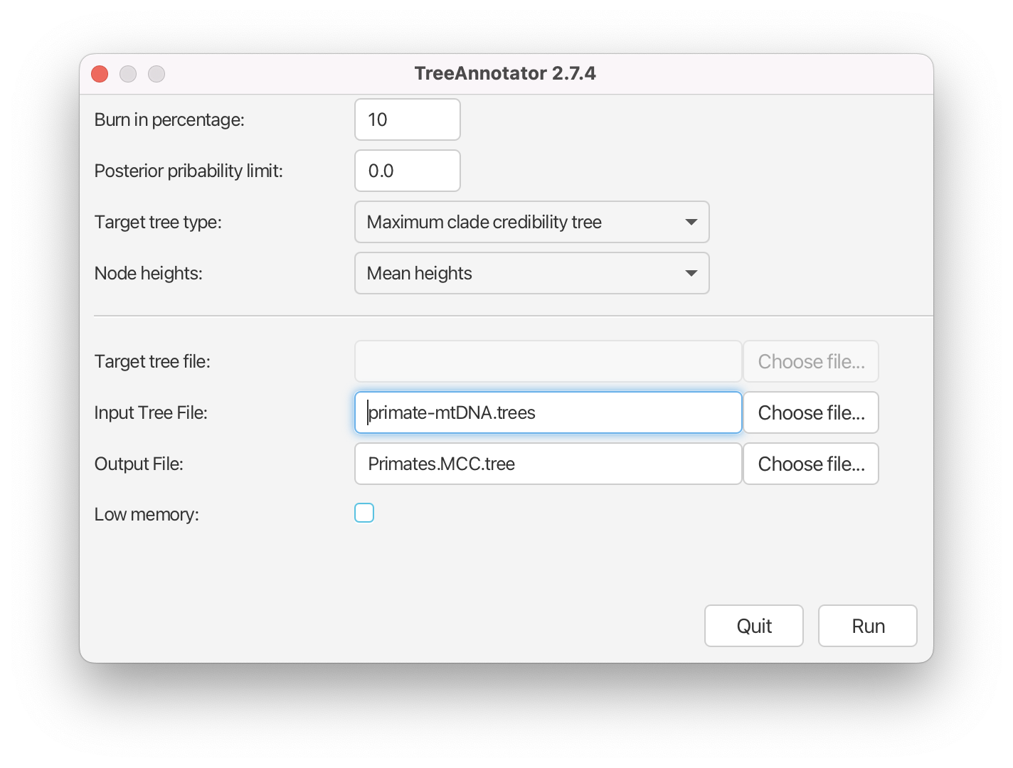
Open TreeAnnotator.
Set the Burnin percentage to 10% to discard the first 10% of trees in the log file.
The next option, the Posterior probability limit, specifies a limit such that if a node is found at less than this frequency in the sample of trees (i.e. has a posterior probability less than this limit), it will not be annotated. For example, setting it to 0.5 means that only nodes seen in the majority (more than 50%) of trees will be annotated. The default value is 0, which we will leave as is, and which means that TreeAnnotator will annotate all nodes.
Leave the Posterior probability limit at the default value of 0.
For the Target tree type option you can either choose a specific tree from a file or ask TreeAnnotator to find a tree in your sample. The default option which we will leave, Maximum clade credibility tree, finds the tree with the highest product of the posterior probability of all its nodes.
Leave the Target tree type at the default value of Maximum clade credibility tree.
Next, select Mean heights for the Node heights. This sets the heights (ages) of each node in the tree to the mean height across the entire sample of trees for that clade.
Select Mean heights in the Node heights drop-down menu.
Finally, we have to select the input tree log file and set an output file.
Click Choose File next to Input Tree File and choose
primate-mtDNA.trees.Set the Output File to
Primates.MCC.tree.
The setup should look as shown in Figure 18. You can now run the program.
Producing CCD0 tree
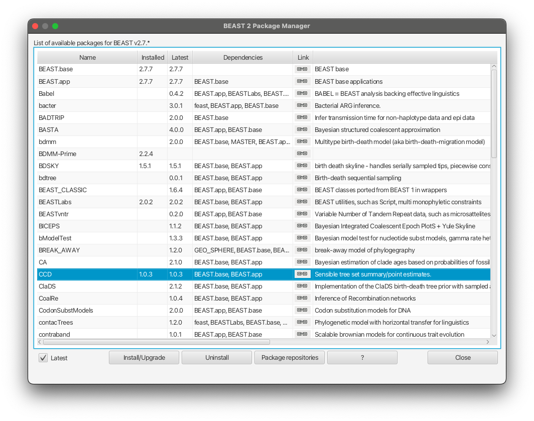
To produce CCD0 summary tree, you will first need to install the CCD package.
Open BEAUTi
Select File -> Manage packages
Select CCD package in the list and select Install/Upgrade Figure 19
Close BEAUTi
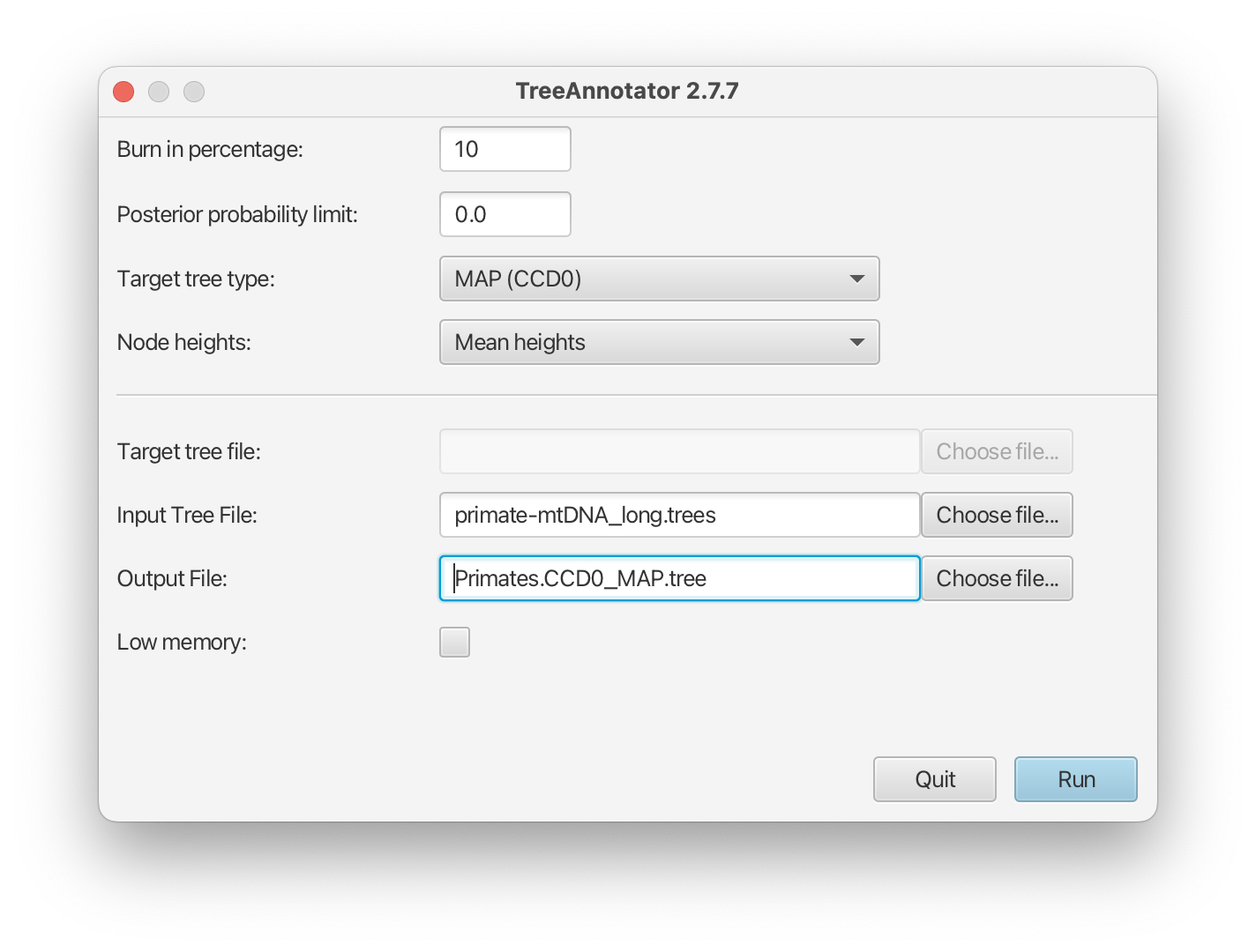
Now you can proceed to make CCD0 tree:
Open TreeAnotator
Repeat all the steps in TreeAnotator as when making the MCC tree, except for Target tree type and Output File.
For Target tree type select MAP(CCD0) from drop down list.
Set the Output File to
Primates.CCD0_MAP.tree.
The setup should look as shown in Figure 20. You can now run the program.
Visualising the tree estimate
Finally, we can visualise the tree with one of the available pieces of software, such as FigTree.
Visualising the MCC tree
Open FigTree. Use File > Open then locate and click on
Primates.MCC.tree.
- Expand Trees options, check Order nodes and select decreasing from the drop-down menu.
- Expand the Tip Labels options and increase the Font Size until it is readable.
- Check the Node Bars checkbox, expand the options and select
height_95%_HPDfrom the Display drop-down menu.- Check the Node Labels checkbox, expand the options and select
posteriorfrom the Display drop-down menu.- Increase the Font Size until it is readable.
- Uncheck the Scale Bar checkbox.
- Check the Scale Axis checkbox, expand the options, check Reverse axis and increase the Font Size.
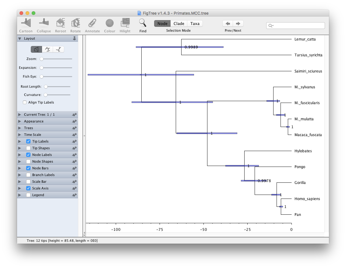
Your tree should now look something like Figure 21. We first ordered the tree nodes. Because there are many ways to draw the same tree ordering nodes makes it easier for us to compare different trees to each other. The scale bars we added represent the 95% HPD interval for the age of each node in the tree, as estimated by the BEAST2 analysis. The node labels we added gives the posterior probability for a node in the posterior set of trees (that is, the trees logged in the tree log file, after discarding the burn-in). We can also use FigTree to display other statistics, such as the branch lengths, the 95% HPD interval of a node etc. The exact statistics available will depend on the model used.
Visualising CCD0 tree
To visualise CCD0 tree, follow the same steps as above, but open the Primates.CCD0_MAP.tree at the first step. Figure 22 shows the resulting tree.
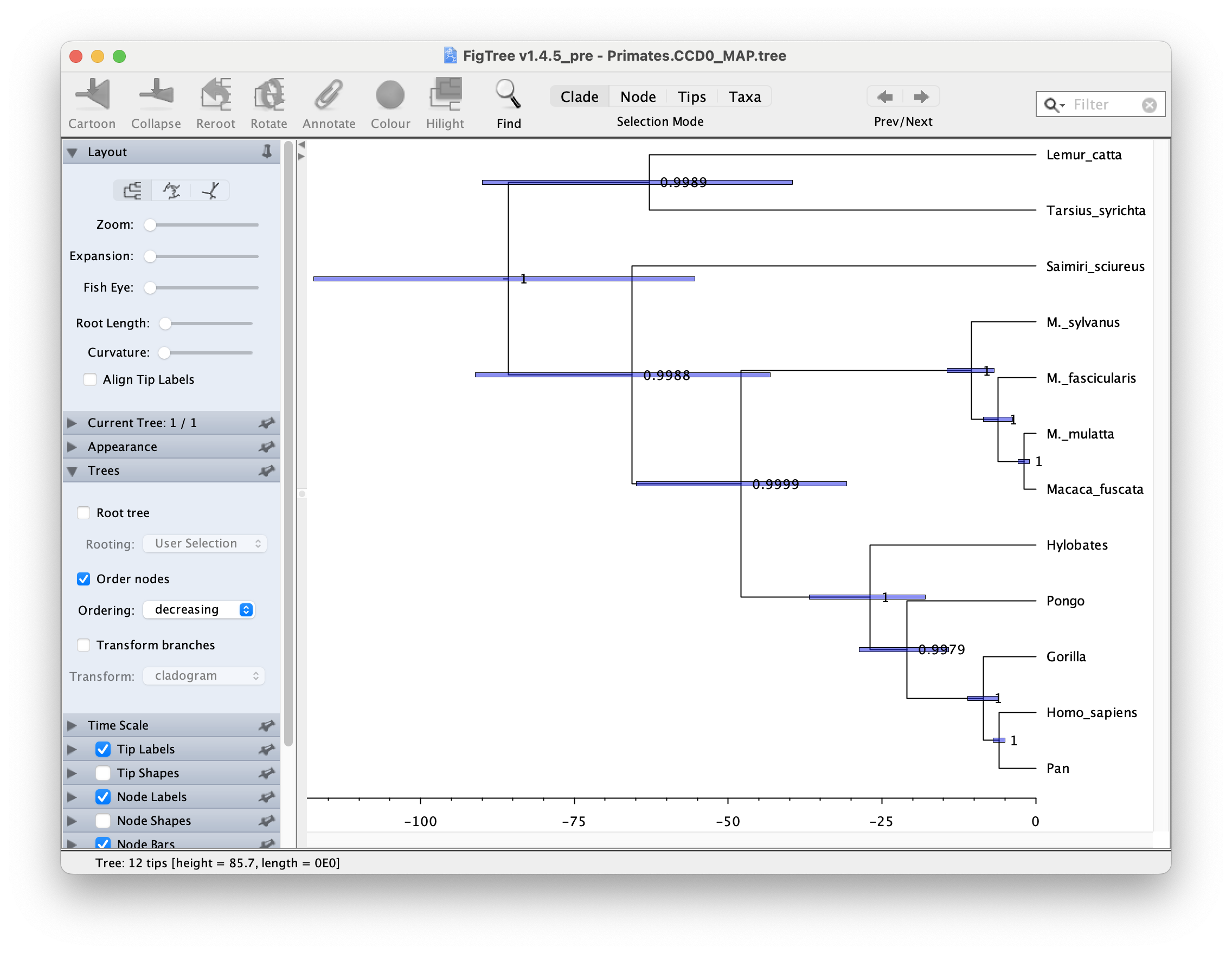
Topics for discussion: The posterior probabilities tell us which clades are highly supported and the scale bars tell us how confident we are about their divergence times.
- Are all clades well-supported? How about their ages?
- Look at the 95% HPD interval for the age of the apes (Hylobates, Pongo, Gorilla, Pan and Homo sapiens). Does the estimated age agree with your prior knowledge?
- What about the divergence time between old-world and new-world monkeys? (Saimiri sciureus is the only new-world monkey in this dataset).
- One of the CCD0 summary method advantages is that it can evaluate tree topologies that were not sampled during the MCMC. In which scenario MCC and CCD0 trees would be (almost) the same? Does it then make sense that our dataset MCC and CCD0 summary tree topologies and clade posterior supports are practically identical?
Visualising tree posteriors (optional)
The MCC tree is one way of summarising the posterior distribution of trees as a single tree, annotated with extra information on some nodes to represent the uncertainty in the tree estimates. Just as summarising the posterior distributions of a continuous parameter as a median and confidence interval throws away a lot of information (such as the shape of the distribution) a lot of information is lost when summarising a set of trees as an MCC tree. However, it is significantly more difficult to visualise the set of posterior trees.
One possibility is to use the program DensiTree. DensiTree does not need a summary tree (so we do not need to run TreeAnnotator prior to using DensiTree) to be able to visualise the estimates.
Open DensiTree. Use File > Load then locate and click on
primate-mtDNA.trees.Expand the Show options and check the Consensus Trees checkbox.
You should now see many lines corresponding to all the individual trees samples by your MCMC chain. You can also clearly see a pattern across all of the posterior trees.
In order to see the support for the topology, select the Central view mode.
Now expand the Clades menu, check the Show clades checkbox and the text checkbox for the Support.
The tree should look as shown in Figure 23.
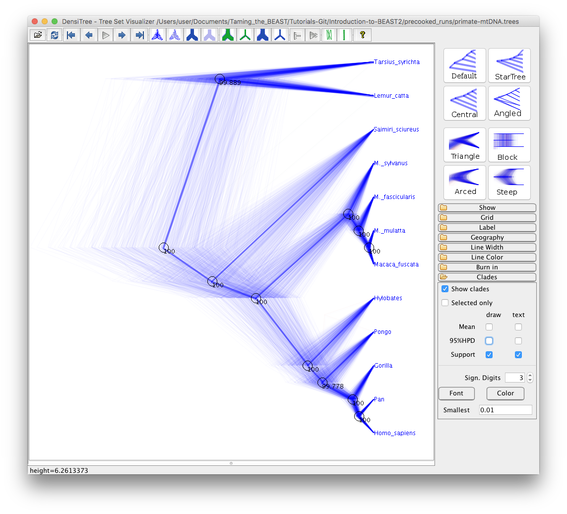
You can also view all of the different clades and their posterior probabilities by selecting Help > View clades. In this particular run there is little uncertainty in the tree estimate with respect to clade grouping, as almost every clade has 100% support.
Topics for discussion: The Yule model for speciation has one parameter (birthRateY.t:tree), representing the speciation rate. This model assumes that there is no extinction and thus that all taxa are sampled.
- What are the units for birthRateY.t:tree? From your analysis, can you figure out the average time it takes for a speciation event to occur? (Have a look at the tracelog).
- Is the Yule model an appropriate model to use here?
- In the dataset there is a much larger sampling proportion for the great apes (4/8 extant species) than for lemurs, tarsiers and new-world monkeys (one species each). Do you think unequal sampling proportions are an issue?
Acknowledgment
The content of this tutorial is based on the Divergence Dating Tutorial with BEAST 2.0 tutorial by Drummond, Rambaut, and Bouckaert.
Useful Links
- Bayesian Evolutionary Analysis with BEAST 2 (Drummond & Bouckaert, 2014)
- BEAST 2 website and documentation: http://www.beast2.org/
- BEAST 1 website and documentation: http://beast.bio.ed.ac.uk
- Join the BEAST user discussion: http://groups.google.com/group/beast-users
- Tree ESS Tutorial
Relevant References
- Bouckaert, R., Heled, J., Kühnert, D., Vaughan, T., Wu, C.-H., Xie, D., Suchard, M. A., Rambaut, A., & Drummond, A. J. (2014). BEAST 2: a software platform for Bayesian evolutionary analysis. PLoS Computational Biology, 10(4), e1003537. https://doi.org/10.1371/journal.pcbi.1003537
- Bouckaert, R., Vaughan, T. G., Barido-Sottani, J., Duchêne, S., Fourment, M., Gavryushkina, A., Heled, J., Jones, G., Kühnert, D., Maio, N. D., Matschiner, M., Mendes, F. K., Müller, N. F., Ogilvie, H. A., Plessis, L. du, Popinga, A., Rambaut, A., Rasmussen, D., Siveroni, I., … Drummond, A. J. (2019). BEAST 2.5: An advanced software platform for Bayesian evolutionary analysis. PLOS Computational Biology, 15(4).
- Berling, L., Klawitter, J., Bouckaert, R., Xie, D., Gavryushkin, A., & Drummond, A. J. (2025). Accurate Bayesian phylogenetic point estimation using a tree distribution parameterized by clade probabilities. PLOS Computational Biology, 21(2), e1012789.
- Drummond, A. J., & Bouckaert, R. R. (2014). Bayesian evolutionary analysis with BEAST 2. Cambridge University Press.
Citation
If you found Taming the BEAST helpful in designing your research, please cite the following paper:
Joëlle Barido-Sottani, Veronika Bošková, Louis du Plessis, Denise Kühnert, Carsten Magnus, Venelin Mitov, Nicola F. Müller, Jūlija Pečerska, David A. Rasmussen, Chi Zhang, Alexei J. Drummond, Tracy A. Heath, Oliver G. Pybus, Timothy G. Vaughan, Tanja Stadler (2018). Taming the BEAST – A community teaching material resource for BEAST 2. Systematic Biology, 67(1), 170–-174. doi: 10.1093/sysbio/syx060