Background

Central among the questions explored in biology are those that seek to understand the timing and rates of evolutionary processes. Accurate estimates of species divergence times are vital to understanding historical biogeography, estimating diversification rates, and identifying the causes of variation in rates of molecular evolution.

This tutorial will provide a general overview of divergence time estimation and fossil calibration using a stochastic branching process and relaxed-clock model in a Bayesian framework. The exercise will guide you through the steps necessary for estimating phylogenetic relationships and dating species divergences using the program BEAST v2.7.x.

This tutorial is available in two formats. A link to a PDF can be found in the column on the left-hand side of this page; the PDF is a more in-depth version of the tutorial, which includes a lot of the background about the fossilized birth-death model. Below is a shorter version which is focused on the more practical aspects of implementing the divergence time analysis.

Programs used in this Exercise

BEAST2 - Bayesian Evolutionary Analysis Sampling Trees 2

BEAST2 is a free software package for Bayesian evolutionary analysis of molecular sequences using MCMC and strictly oriented toward inference using rooted, time-measured phylogenetic trees (Drummond et al., 2006; Drummond & Rambaut, 2007; Bouckaert et al., 2014). The development and maintenance of BEAST is a large, collaborative effort and the program includes a wide array of different types of analyses. This tutorial uses the BEAST v2.7.4.

BEAUti - Bayesian Evolutionary Analysis Utility

BEAUti2 is a utility program with a graphical user interface for creating BEAST2 input files which must be written in the XML. This application provides a clear way to specify priors, partition data, calibrate internal nodes, etc.

Both BEAST2 and BEAUti2 are Java programs, which means that the exact same code runs, and the interface will be the same, on all computing platforms. The screenshots used in this tutorial are taken on a Mac OS X computer; however, both programs will have the same layout and functionality on both Windows and Linux. BEAUti2 is provided as a part of the BEAST2 package so you do not need to install it separately.

TreeAnnotator

TreeAnnotator is used to summarize the posterior sample of trees to produce a maximum clade credibility tree and summarize the posterior estimates of other parameters that can be easily visualized on the tree (e.g. node height). This program is also useful for comparing a specific tree topology and branching times to the set of trees sampled in the MCMC analysis.

Tracer

Tracer is used for assessing and summarizing the posterior estimates of the various parameters sampled by the Markov Chain. This program can be used for visual inspection and assessment of convergence and it also calculates 95\% credible intervals (which approximate the 95\% highest posterior density intervals) and effective sample sizes (ESS) of parameters. We will be using Tracer v.

FigTree

FigTree is an excellent program for viewing trees and producing publication-quality figures. It can interpret the node-annotations created on the summary trees by TreeAnnotator, allowing the user to display node-based statistics (e.g. posterior probabilities) in a visually appealing way.

Practical: Divergence Time Estimation

This tutorial will walk you through an analysis of the divergence times of the bears. The occurrence times of 14 fossil species are integrated into the tree prior to impose a time structure on the tree and calibrate the analysis to absolute time. Additionally, an uncorrelated, lognormal relaxed clock model is used to describe the branch-specific substitution rates.

The Data

The data files and pre-cooked output files can be downloaded from the panel on the left. The analysis in this tutorial includes data from several different sources.

We have molecular sequence data for eight extant species, which represent all of the living bear taxa. The sequence data include interphotoreceptor retinoid-binding protein (irbp) sequences (in the file bears_irbp_fossils.nex) and 1000 bps of the mitochondrial gene cytochrome b (in the file bears_cytb_fossils.nex). If you open either of these files in your text editor or alignment viewer, you will notice that there are 22 taxa listed in each one, with most of these taxa associated with sequences that are entirely made up of missing data (i.e., ?????). This is because the NEXUS files also contain the names of 14 fossil species, that we will include in our analysis as calibration information for the fossilized birth-death process.

For these extinct taxa, we must provide an occurrence time for each taxon sampled from the fossil record. This information is obtained from the literature or fossil databases like the Paleobiology Database or the Fossil Calibration Database, or from your own paleontological expertise.

The final source of data required for our analysis is some information about the phylogenetic placement of the fossils. This prior knowledge can come from previous studies of morphological data and taxonomy. Ideally, we would like to know exactly where in the phylogeny each fossil belongs. However, this is uncommon for most groups in the fossil record. For the bear species in our analysis, we do have some prior knowledge about their relationships. Four out of five of the clades we will define in the NEXUS file bears_cytb_fossils.nex as taxsets in the sets block. The one clade that is not included in the data file will be created using the BEAUti options.

Creating the Analysis File with BEAUti

Creating a properly-formatted BEAST XML file from scratch is not a simple task. However, BEAUti provides a simple way to navigate the various elements specific to the BEAST XML format.

Begin by starting BEAUti2.

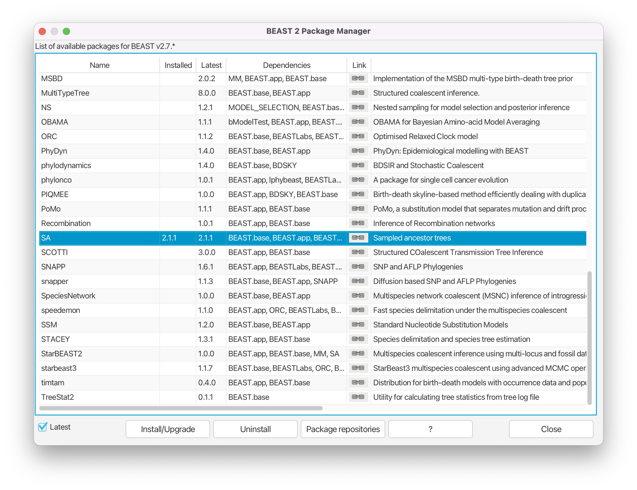
Install BEAST2 packages

Next, we have to install the BEAST 2 packages that are needed for this analysis. The packages that we will use called SA (Sampled Ancestors) and ORC (Optimized Relaxed Clock).

Open the Package Manager by navigating to File > Manage Packages in the menu. Install the SA package by selecting it and clicking the Install/Upgrade button. Do the same for the ORC package. Close the BEAST2 Package Manager and restart BEAUti to fully load the packages.

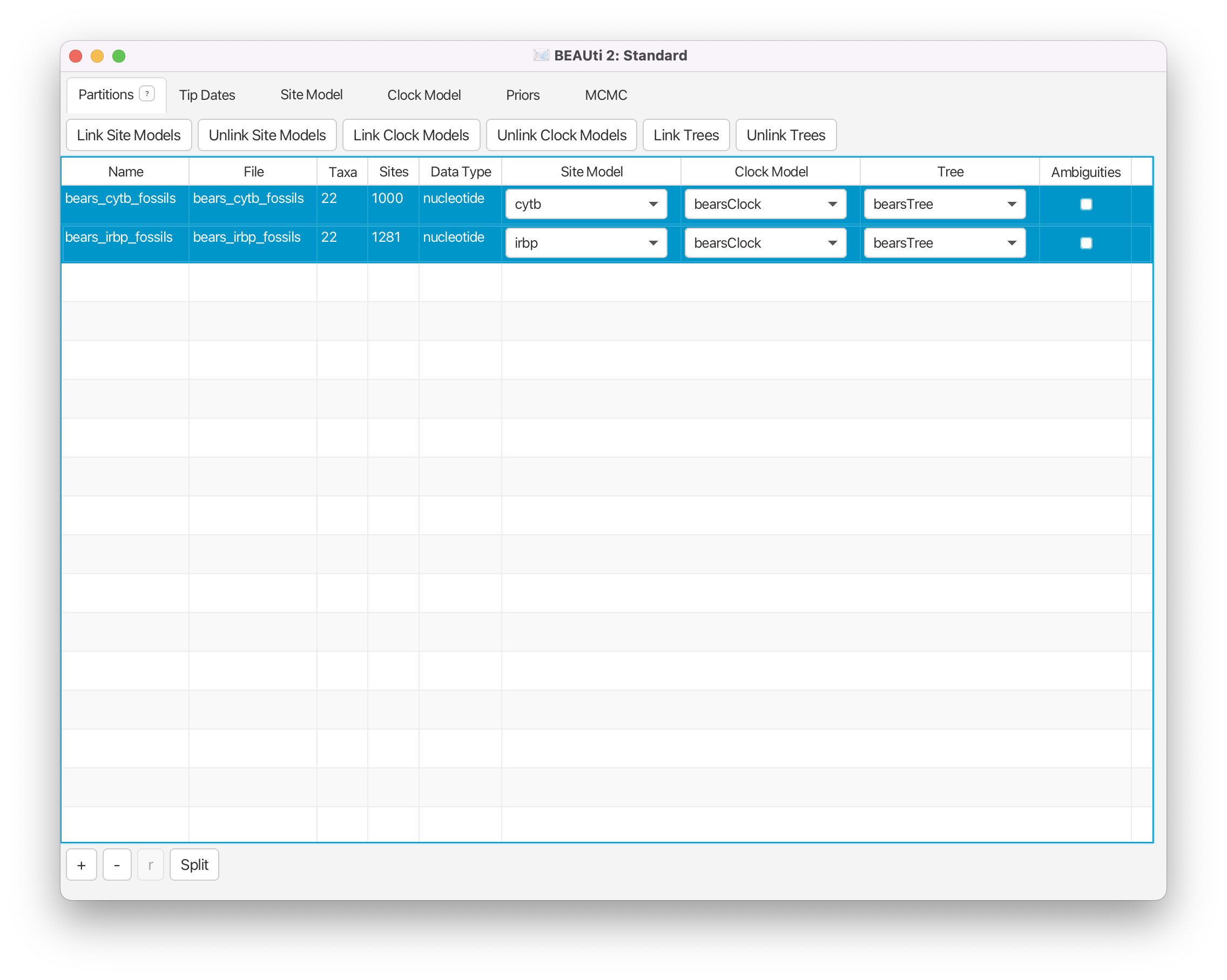
Import Alignments

Next we will load the alignment files for each of our genes from our NEXUS files.

Navigate to the Partitions window. Using the menu commands File > Import Alignment, import the data files bears_irbp_fossils.nex and bears_cytb_fossils.nex.

Now that the data are loaded into BEAUti, we can unlink the site models, link the clock models, link the trees, and rename these variables so they are easier to understand in the output files.

Highlight both partitions (using shift and click) and click on Unlink Site Models to assume different models of sequence evolution for each gene (the partitions are typically already unlinked by default). Click the Link Clock Models button so that the two genes have the same relative rates of substitution among branches. Click Link Trees to ensure that both partitions share the same tree topology and branching times.

Double click on the site model for the cytochrome b gene (bears_cytb_fossils). Rename this to cytb. (Note that you may have to hit the return or enter key after typing in the new label for the new name to be retained.) Do the same for the site model for the other gene, calling it irbp. Rename the clock model to bearsClock, and rename the tree to bearsTree.

Set Tip Dates

We must indicate that we have sequentially sampled sequences, and when those sequences were collected. We will indicate that the dates are in years, even though they are in fact in units of millions of years. This is because the units themselves are arbitrary and this scale difference will not matter. Additionally, we will tell BEAUti that the “zero time” of our tree is the present and the ages we are providing are the number of years before the present.

Navigate to the Tip Dates panel. Toggle on the Use tip dates option. Change Dates specified to year Before the present.

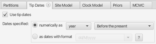
Conveniently, we can specify that our dates are included in the taxon names, so that BEAUti can extract them for us using the Auto-configure option.

Click on the Auto-configure button. Tell BEAUti to use everything after the last _, then click OK.

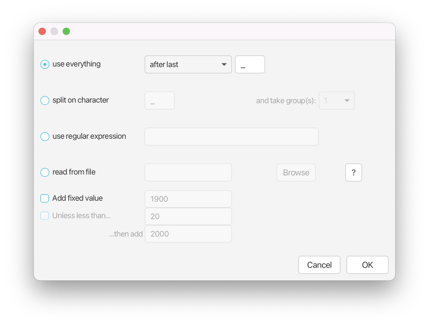
You should now see that the tip ages have been filled in for all of the fossil taxa and that the same age is listed in the Date and Height column for each species.

Specify the Site Model

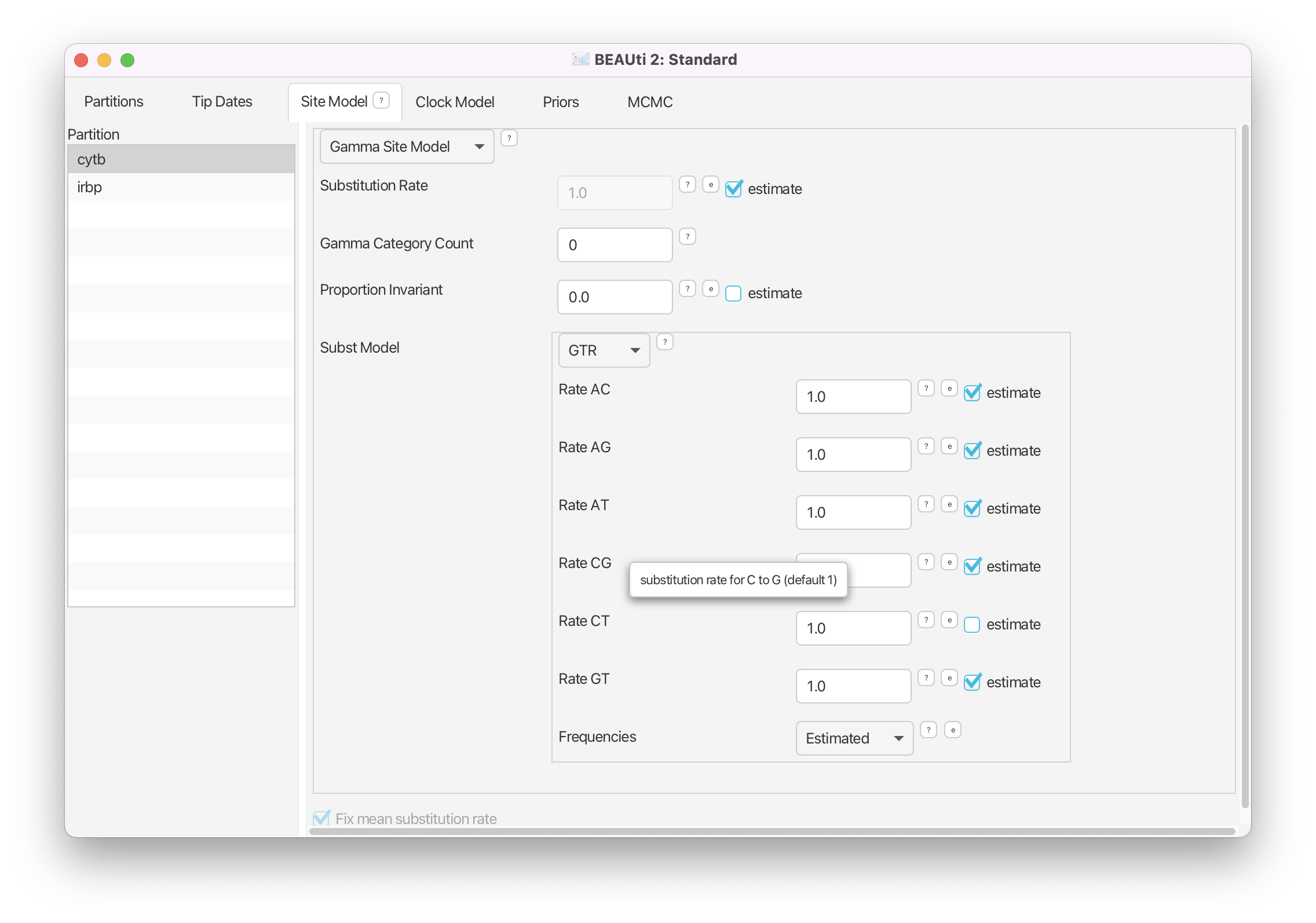
The molecular sequence data sampled for each extant bear species are from two different genes: the mitochondrial cytochrome b gene (cytb) and the nuclear interphotoreceptor retinoid-binding protein gene (irbp). We will partition these loci into two separate alignments and apply different models of sequence evolution to each one. For the cytb gene, we will apply a general-time reversible model with homogeneous rates across sites: GTR. For the nuclear gene irbp, we will assume a 2-rate model where transitions and transversions happen at different rates, and that the rates vary across the alignment according to a mean-one gamma distribution: HKY+Gamma.

Navigate to the Site Model window. Select the cytb gene and change the Subst Model to GTR. Toggle on estimate for the Substitution Rate.

Select the irbp gene and change the Subst Model to HKY. To indicate gamma-distributed rates, set the Gamma Category Count to 4. Check that the Shape parameter is set to estimate. Toggle on estimate for the Substitution Rate.

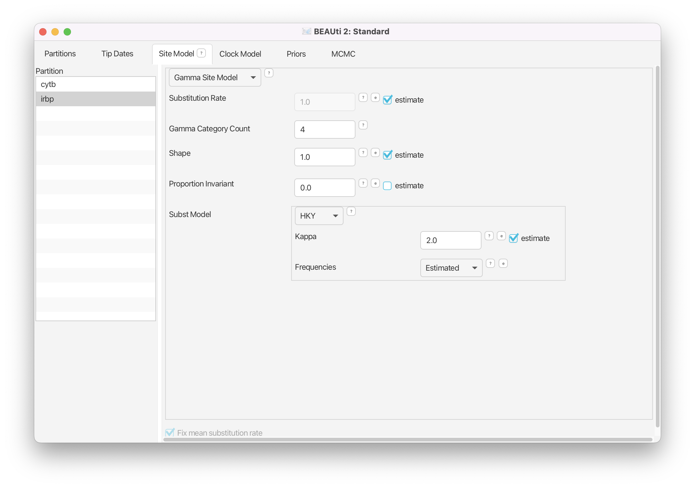
Now both models are fully specified for the unlinked genes. Note that Fix mean substitution rate is always specified and we also have indicated that we wish to estimate the substitution rate for each gene. This means that we are estimating the relative substitution rates for our two loci.

The Clock Model

Here, we can specify the model of lineage-specific substitution rate variation. The default model in BEAUti is the Strict Clock. For this analysis we will use an uncorrelated, lognormal model of branch-rate variation. The Optimized Relaxed Clock option (provided by the ORC package) assumes that the substitution rates associated with each branch are independently drawn from a single, discretized lognormal distribution (Drummond et al., 2006).

Navigate to the Clock Model window. Change the clock model to Optimized Relaxed Clock.

The uncorrelated relaxed clock models in BEAST2 are discretized for computational feasibility. This means that for any given parameters of the lognormal distribution, the probability density is discretized into some number of discrete rate bins. Each branch is then assigned to one of these bins. By default, BEAUti sets the Number Of Discrete Rates to -1. This means that the number of bins is equal to the number of branches. The fully specified Clock Model assumes that the rates for each branch are drawn independently from a single lognormal distribution. The mean of the rate distribution will be estimated, thus we can account for uncertainty in this parameter by placing a prior distribution on its value.

Priors on Parameters of the Site Models

In the Priors panel we will begin by specifying priors for the parameters associated with the site models. Since we partitioned the two genes, there are parameters for the two different models:

• exchangeability rates for the GTR model (rateAC.s:cytb, rateAG.s:cytb, …, rateGT:.s:cytb)
• the transition-transversion rate ratio (kappa.s:irbp) and the shape parameter of the gamma distribution on site rates (gammaShape.s:irbp)
• The equilibrium nucleotide frequencies for both partitions (freqParameter.s:cytb and freqParameter.s:irbp)

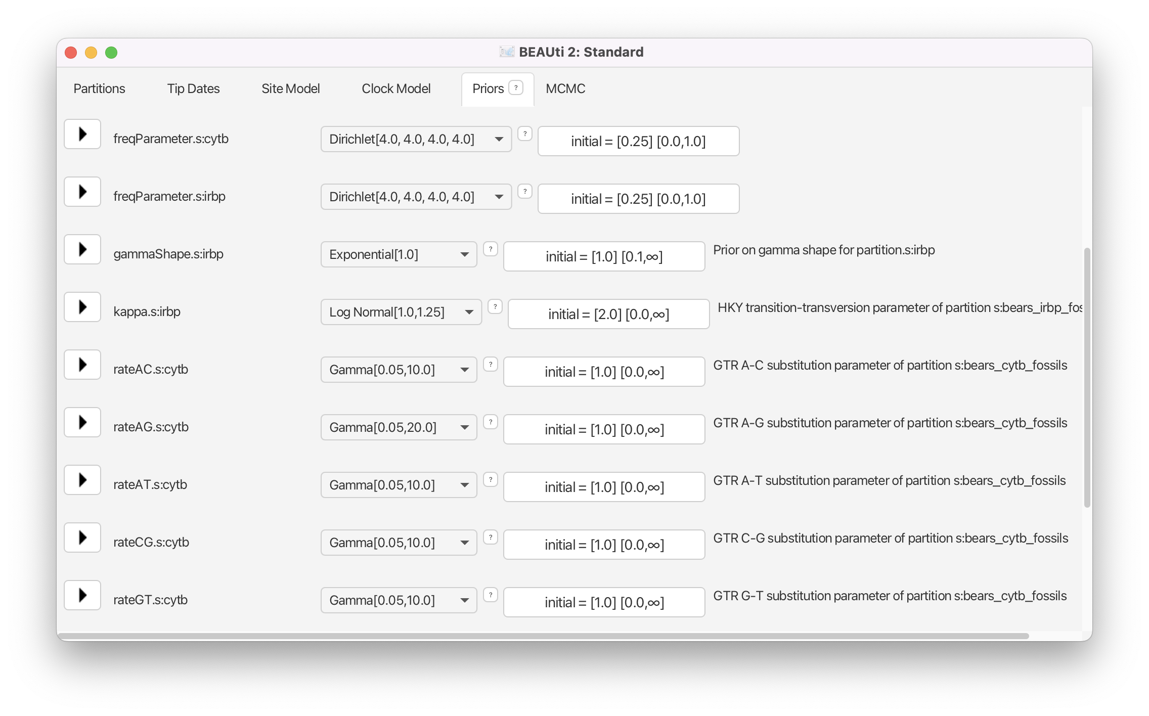
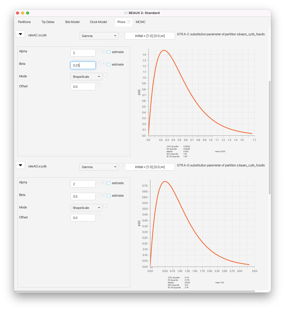
We will keep the default priors for the HKY model on the evolution of irbp. The default gamma priors on the GTR exchangeability rates for the cytb gene place a lot of prior density on very small values. For some datasets, the sequences might not be informative for some of the rates, consequentially the MCMC may propose values very close to zero and this can induce long mixing times. Because of this problem, we will alter the gamma priors on the exchangeability rates. For each one, we will keep the expected values as in the default priors. The default priors assume that transitions (A <-> G or C <-> T) have an expected rate of 1.0. Note that BEAUti automatically fixes the parameter rateCT to be equal 1.0 in the Site Model window, thus this parameter isn’t present in the Priors window. For all other rates, transversions, the expected value of the priors is lower: 0.5. In BEAST2, the gamma distribution is parameterized by a shape parameter (Alpha) and a scale parameter (Beta). Under this parameterization, the expected value for any gamma distribution is: $\mathbb{E}(x) = \alpha\beta$. To reduce the prior density on very low values, we can increase the shape parameter and then we have to adjust the scale parameter accordingly.

Navigate to the Priors window. Begin by changing the gamma prior on the transition rate rateAG.s:cytb. Clicking on the $\blacktriangleright$ next to this parameter name to reveal the prior options. Change the parameters: Alpha = 2 and Beta = 0.5. Then change all of the other rates, for rateAC.s, rateAT.s, rateCG.s, and rateGT.s, to Alpha = 2 and Beta = 0.25.

Priors for the Clock Model

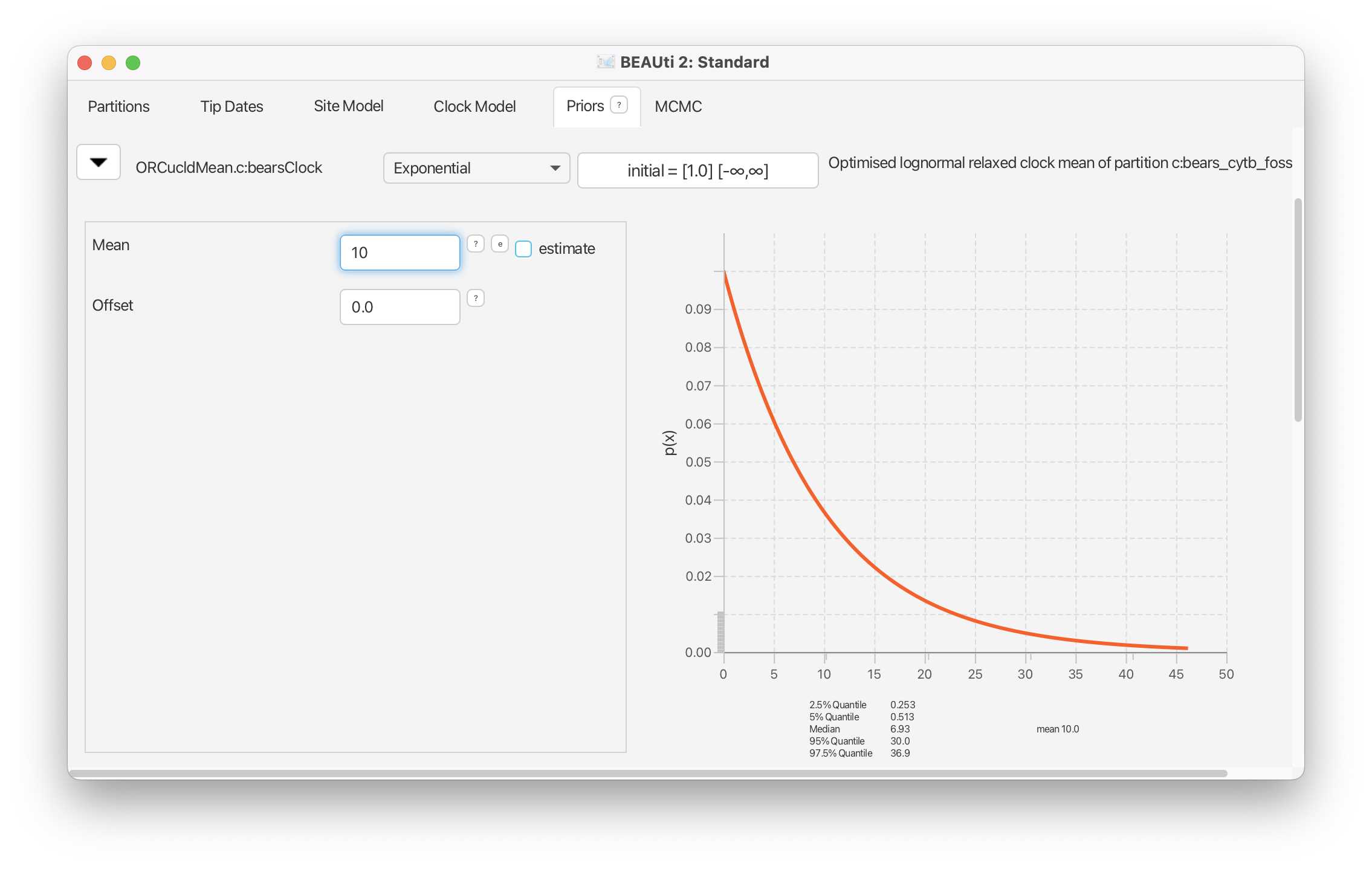
Since we are assuming that the branch rates are drawn from a lognormal distribution, this induces two hyperparameters: the mean and standard deviation (ORCucldMean.c and ORCsigma.c respectively). By default, the prior distribution on the ORCucldMean.c parameter is an improper, uniform distribution on the interval $(0,\infty)$. Instead, we will change this to an exponential prior.

Reveal the options for the prior on ORCucldMean.c by clicking on the $\blacktriangleright$. Change the prior density to an Exponential with a mean of 10.0.

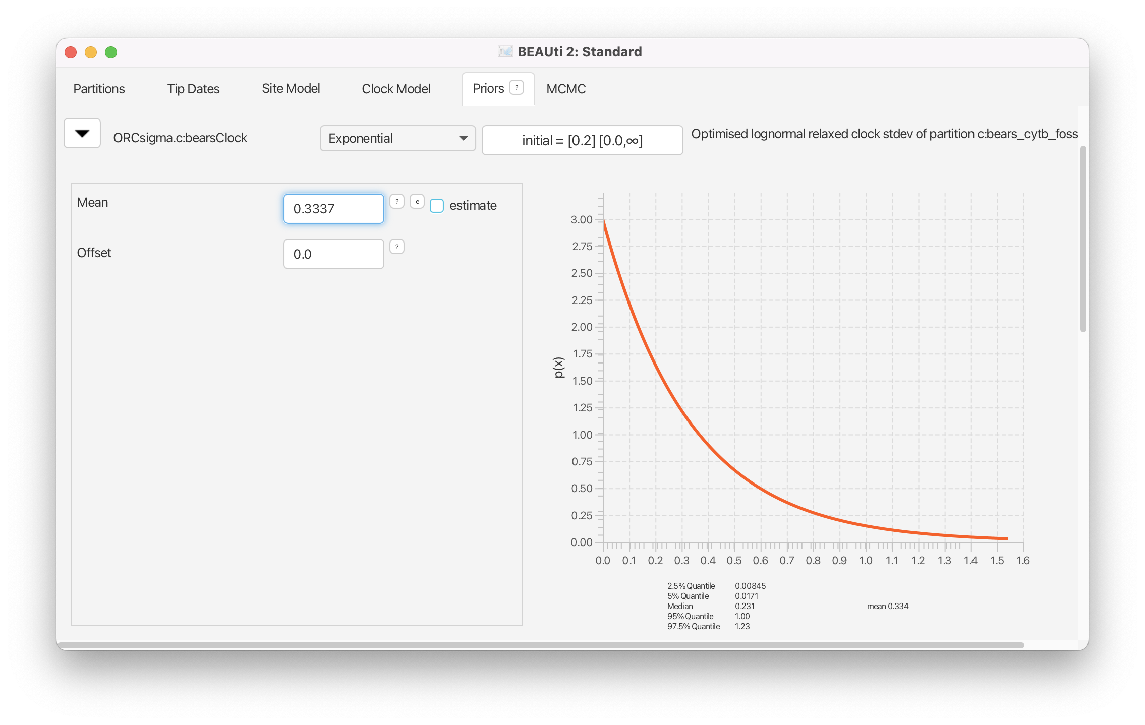
The other parameter of our relaxed-clock model is, by default, assigned a gamma prior distribution. However, we have a strong prior belief that the variation in substitution rates among branches is low, since some previous studies have indicated that the rates of molecular evolution in bears is somewhat clock-like (Krause et al., 2008). Thus, we will assume an exponential prior distribution with 95% of the probability density on values less than 1 for the ORCsigma.c parameter.

Reveal the options for the prior on ORCsigma.c by clicking on the $\blacktriangleright$. Change the prior density to an Exponential with a mean of 0.3337.

The Tree Prior

Next we will specify the prior distribution on the tree topology and branching times in the Priors panel. Here is where we specify that we want to use the fossilized birth-death process.

Change the tree model for Tree.t:bearsTree to Fossilized Birth Death Model. Reveal the options for the prior on Tree.t by clicking on the $\blacktriangleright$.

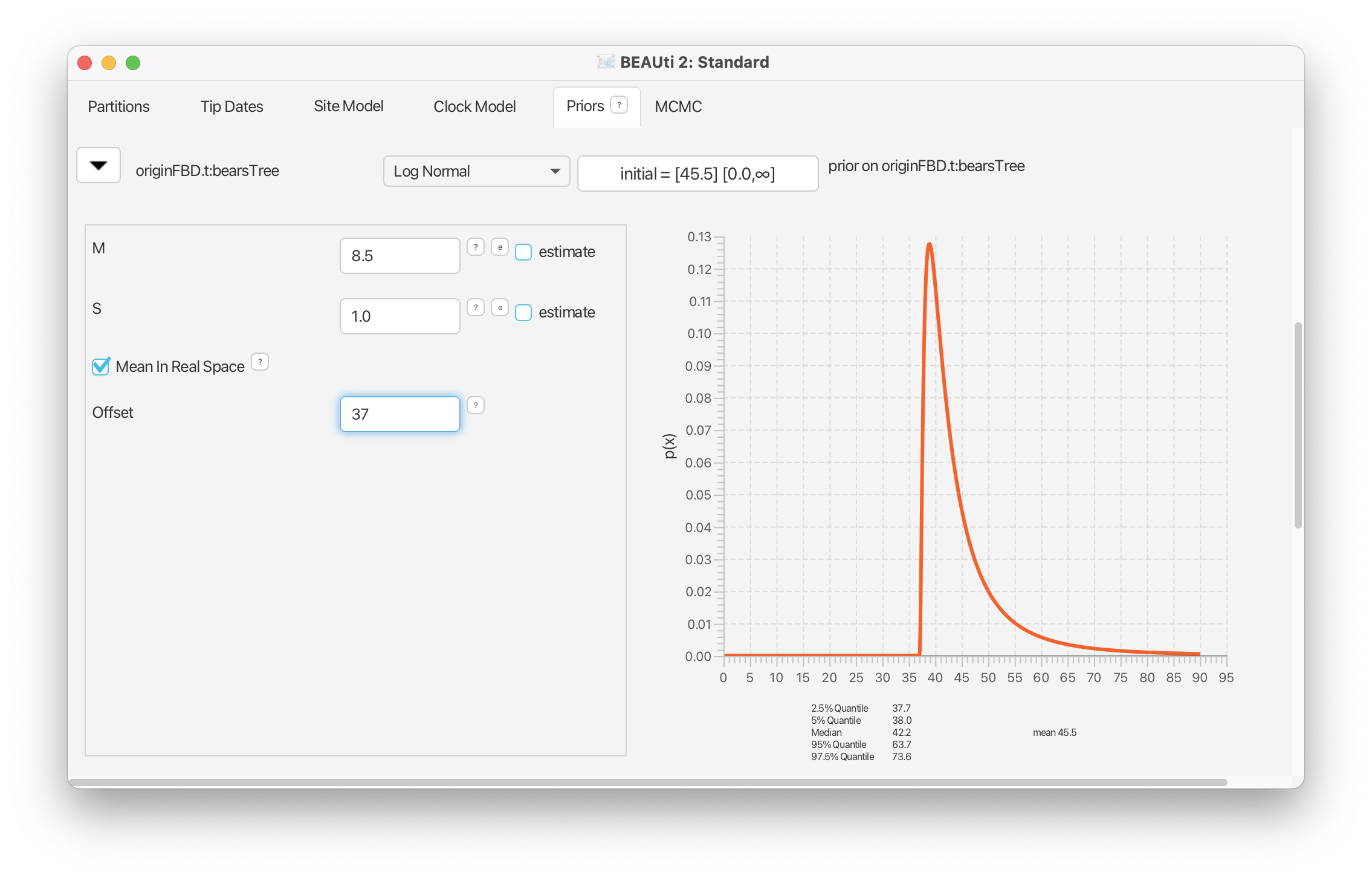
This model, like any branching process (i.e., constant rate birth-death, Yule) can be conditioned on either the origin time or the root age. If you know that all of the fossils in your dataset are crown fossils—descendants of the MRCA of all the extant taxa—and you have some prior knowledge of the age of the clade, then it is reasonable to condition the FBD on the root. Alternatively, if the fossils in your analysis are stem fossils, or can only reliably be assigned to your total group, then it is appropriate to condition on the origin age. For this analysis, we have several bear fossils that are considered stem fossils, thus we will condition on the origin age. Previous studies (dos Reis et al., 2012) estimated an age of approximately 45.5 My for the MRCA of seals and bears. We will use this time as a starting value for the origin.

Set the starting value of the Origin to 45.5 and make sure that the estimate box is checked. (You may have to expand the width of the BEAUti window to see the check-boxes for these parameters.)

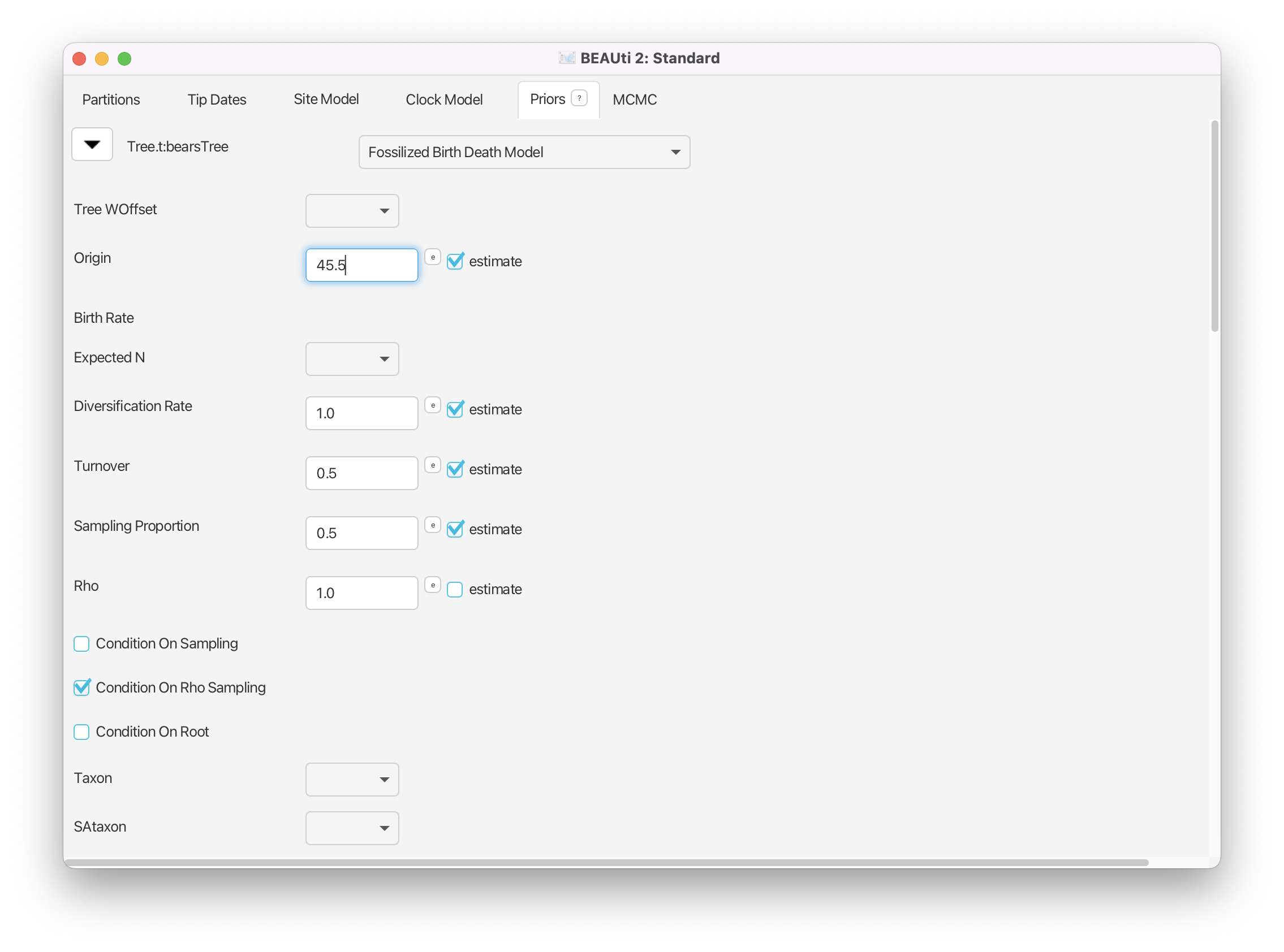
Since we are estimating the origin parameter, we must assign a prior distribution to it. We will assume that the origin time is drawn from a lognormal distribution with an expected value (mean) equal to 45.5 My and a standard deviation of 1.0. We will use the Mean in Real Space option, to indicate that the mean value we enter is the expected value in real space rather than log-transformed space, and set the value to 8.5 My.

Reveal the options for the prior on originFBD.t by clicking on the $\blacktriangleright$. Change the prior distribution to Log Normal. Check the box marked Mean In Real Space and set the mean M equal to 8.5 and the standard deviation S to 1.0. Set the Offset of the lognormal distribution to equal the age of the oldest fossil: 37.0.

The diversification rate is $d = \lambda-\mu$. We would expect that this value is fairly small, particularly since we have few extant species and many fossils. Therefore, an exponential distribution is a reasonable prior for this parameter as it places the highest probability on zero. For this analysis we will assume $d\sim \exp(1.0)$. The exponential distribution’s only parameter is called the rate parameter (denoted $\nu$) and it controls both the mean and variance of the distribution (here $\nu=1$).

Reveal the options for the prior on diversificationRateFBD.t by clicking on the $\blacktriangleright$. Change the prior distribution to Exponential with a Mean equal to 1.0.

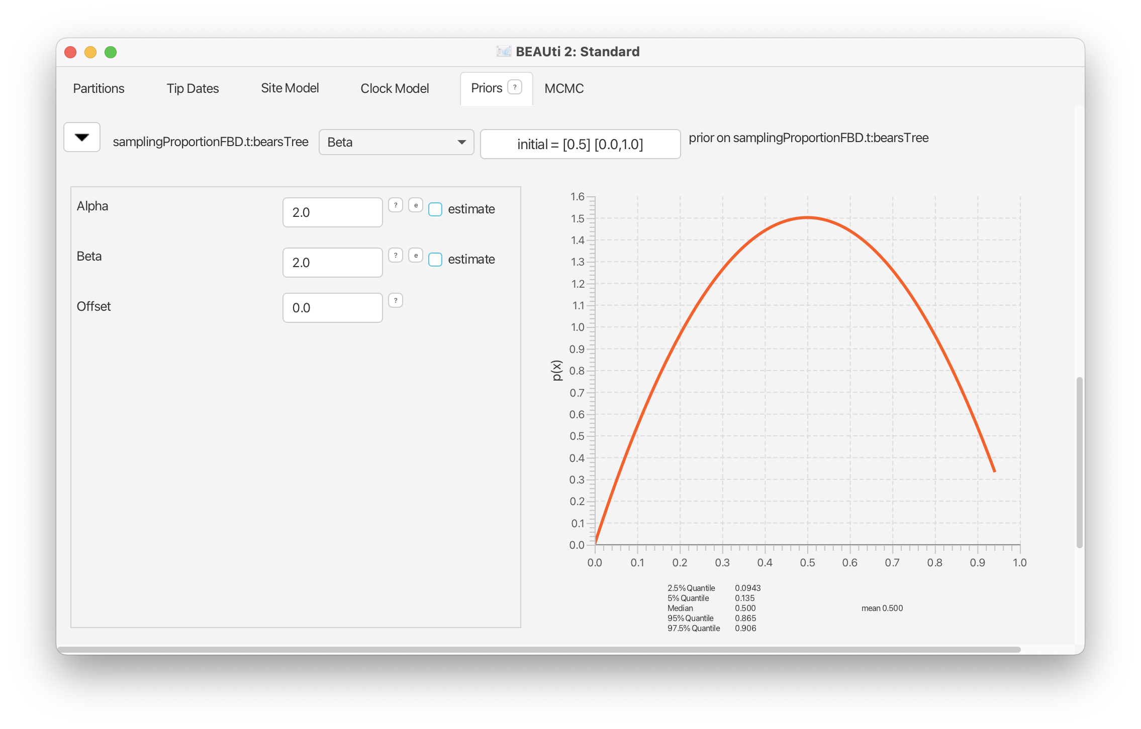
The sampling proportion is the probability of observing a fossil of a given lineage. This parameter is a function of the extinction rate ($\mu$) and the fossil recovery rate ($\psi$): $s=\psi / (\mu+\psi)$. Let’s say that we have prior knowledge that this parameter is approximately equal to 0.5, and that we wish extreme values (very close to 0 or 1) to have low probability. This prior density can be described with a beta distribution. The beta distribution is a probability density over values between 0 and 1 and is parameterized by two values, called $\alpha$ and $\beta$. For this prior we will set $\alpha=\beta=2$.

Reveal the options for the prior on samplingProportionFBD.t by clicking on the $\blacktriangleright$. Change the prior distribution to Beta with Alpha equal to 2.0 and Beta equal to 2.0.

The parameter $\rho$ (Rho) represents the probability of sampling a tip in the present. For most birth-death processes, it is helpful to be able to fix or place a very strong prior on one of the parameters ($\lambda, \mu, \rho, \psi$) because of the strong correlations that exist among them. Typically, we may have the most prior knowledge about the proportion of sampled extant species ($\rho$). We know that there are only 8 species of bear around today, and we have sequence data representing each of these species, so we can fix $\rho=1$. As a result, we do not need to specify a prior for this parameter. This is already the default setting of the fossilized birth-death process and there is nothing for us to do here (see Figure 12 to chck that Rho is set to 1 and not estimated).

The turnover parameter represents the relative rate of extinction: $r = \mu/\lambda$. This parameterisation of the birth-death model assumes that $\mu < \lambda$, thus this parameter is always $r < 1$. It is challenging to define an appropriate prior for the turnover parameter and we will simply assume that all values on the interval [0,1] have equal probability. Thus, we can leave the default prior, a Uniform(0,1), on this parameter.

Creating Taxon Sets

Since some of the relationships between fossil and living bears are well understood (from previous analyses of molecular and morphological data), we can incorporate this prior information by creating monophyletic taxon sets in BEAUti. In the absence of morphological data for our extinct species, if we do not impose any phylogenetic structure on them, they will have equal probability of attaching to any branch in the tree. Given that previous studies have provided information about the relationships of fossil bears, we can limit the MCMC to only place these fossil bears within their known groups.

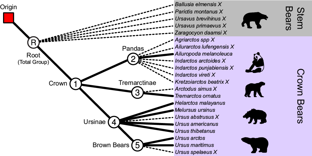
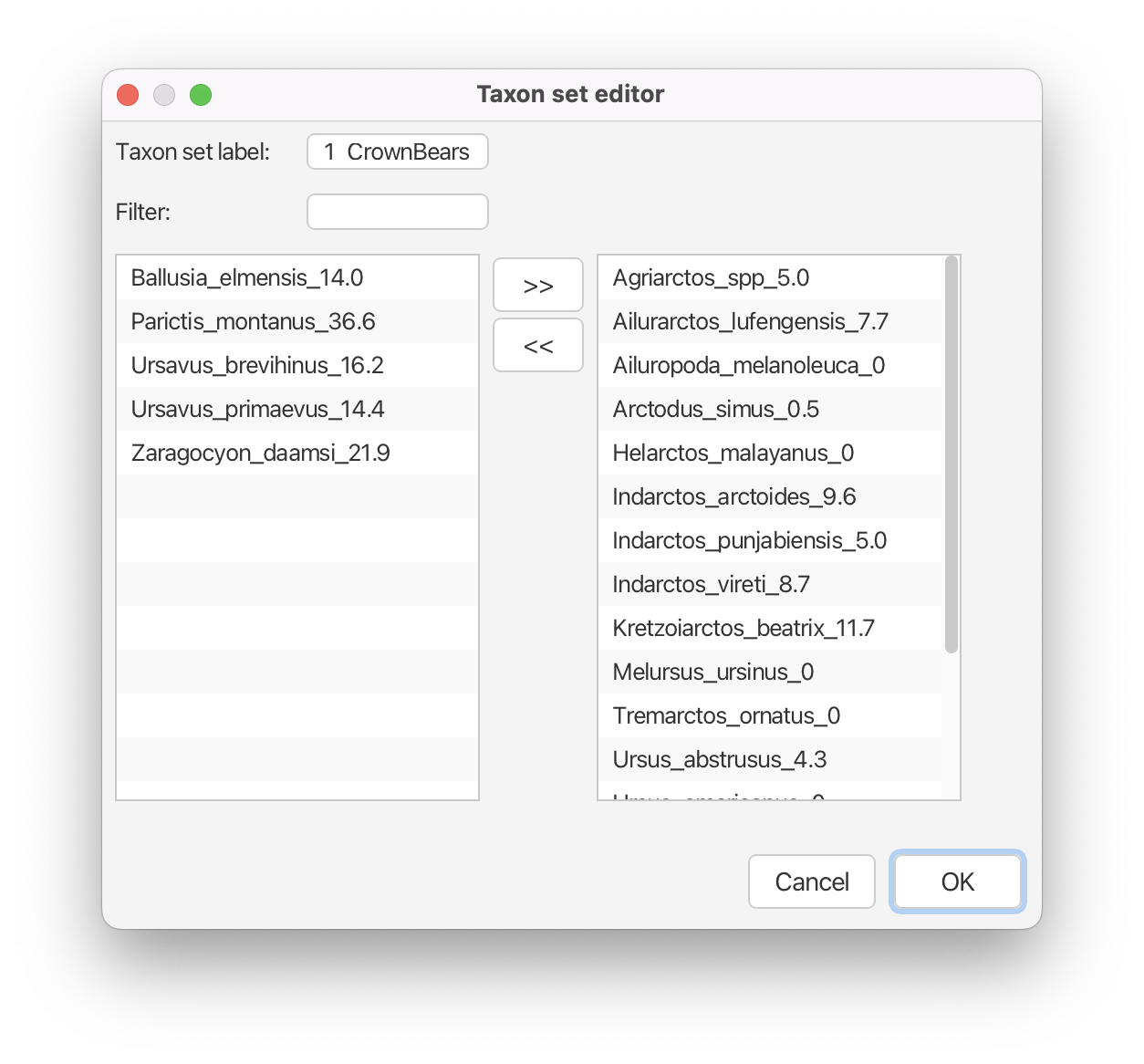
There are five distinct clades within the phylogeny of bears that we can define, and four out of five of these clades are defined as taxon sets in one of the NEXUS files containing our sequences (bears_cytb_fossils.nex). The taxa represented in our dataset are in the total group of bears. This includes all of the fossils that diverged before the most-recent-common-ancestor (MRCA) of all living bears. These early diverging fossils are stem lineages.

Four out of five of the taxon sets needed for this analysis have already been specified in one of the NEXUS files containing our sequences. The first taxon set is the crown bears, shown below. The crown bears include all living species of bears and all the fossils that are descended from the MRCA of living taxa.

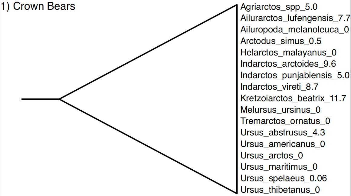
You can open and view the automatically generated BEAUti taxon set for the crown bears by clicking the 1_CrownBears.prior button.

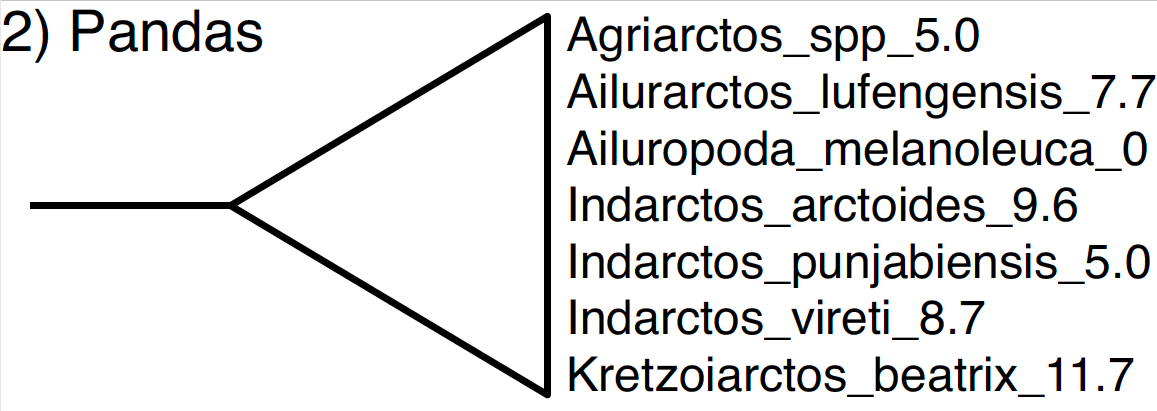
The second node defined in our NEXUS file is the MRCA of all species within the subfamily Ailuropodinae. This group includes the giant panda (Aliuropoda melanoleuca) and six fossil relatives.

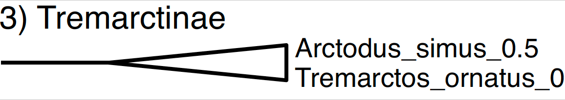
The subfamily Tremarctinae includes only the extant spectacled bear (Tremarctos ornatus) and the short-faced bear (Arctodus simus). The occurrence time of the short-faced bear is only 500,000 years ago since it is known from the Pleistocene.

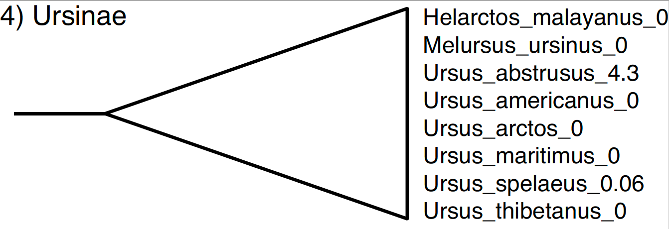
The subfamily Ursinae comprises all of the species in the genus Ursus (including two fossil species) as well as the sun bear (Helarctos malayanus) and the sloth bear (Melursus ursinus).

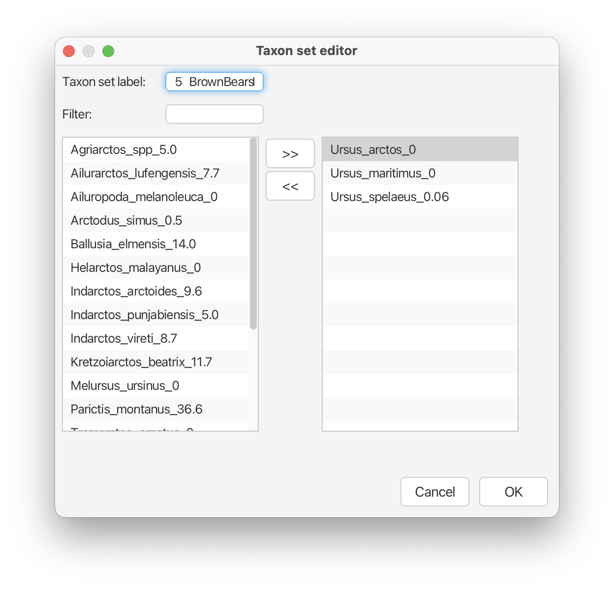
Finally, multiple studies using molecular data have shown that the polar bear (Ursus maritimus) and the brown bear (Ursus arctos) are closely related. Furthermore, phylogenetic analyses of ancient DNA from Pleistocene sub-fossils concluded that the cave bear (Ursus spelaeus) is closely related to the polar bear and the brown bear. This taxon set is not included in our NEXUS file, so we will define it using BEAUti.

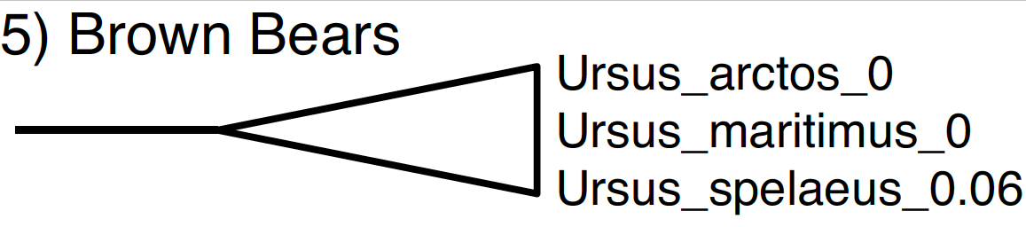
Create a new taxon set for node 5 by clicking the + Add Prior button and select MRCA prior in the pop-up option box. Label this taxon set 5_BrownBears. Move Ursus arctos, Ursus maritimus and Ursus spelaeus to the right-hand column, and click OK. Back in the Priors window, check the box labeled monophyletic for node 5.

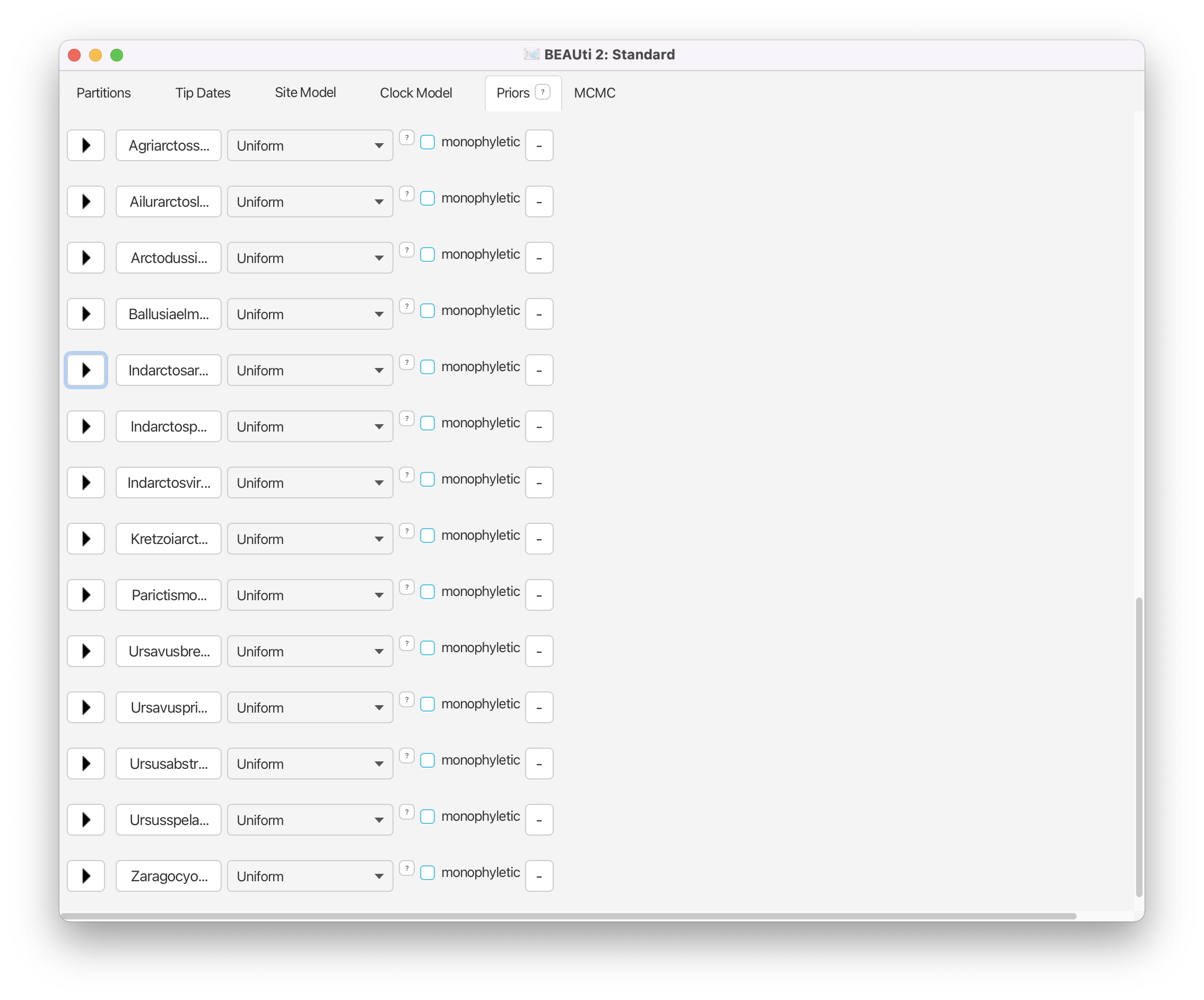
At this point, there should be five monophyletic taxon sets listed in the Priors window.

Sampling the fossil ages

In order to sample the age of fossil specimens, we need to specify prior distributions for these ages. The age ranges for our fossil samples are shown in the table below, modified from Table S.3 in the supplemental appendix of (Heath et al., 2014).

Fossil species	Age range (My)	Citation
Parictis montanus	33.9-37.2	(Clark & Guensburg, 1972; Krause et al., 2008)
Zaragocyon daamsi	20-22.8	(Ginsburg & Morales, 1995; Abella et al., 2012)
Ballusia elmensis	13.7-16	(Ginsburg & Morales, 1998; Abella et al., 2012)
Ursavus primaevus	13.65-15.97	(Andrews & Tobien, 1977; Abella et al., 2012)
Ursavus brevihinus	15.97-16.9	(Heizmann et al., 1980; Abella et al., 2012)
Indarctos vireti	7.75-8.7	(Montoya et al., 2001; Abella et al., 2012)
Indarctos arctoides	8.7-9.7	(Geraads et al., 2005; Abella et al., 2012)
Indarctos punjabiensis	4.9-9.7	(Baryshnikov, 2002; Abella et al., 2012)
Ailurarctos lufengensis	5.8-8.2	(Jin et al., 2007; Abella et al., 2012)
Agriarctos spp.	4.9-7.75	(Abella et al., 2011; Abella et al., 2012)
Kretzoiarctos beatrix	11.2-11.8	(Abella et al., 2011; Abella et al., 2012)
Arctodus simus	0.012-2.588	(Churcher et al., 1993; Krause et al., 2008)
Ursus abstrusus	1.8-5.3	(Bjork, 1970; Krause et al., 2008)
Ursus spelaeus	0.027-0.25	(Loreille et al., 2001; Krause et al., 2008)

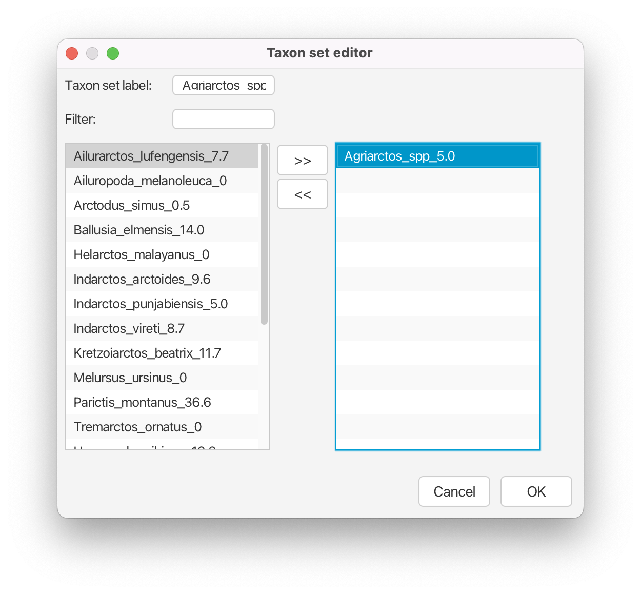
Since we have no prior knowledge on where the true age of the specimen lies within the range, we will use uniform distributions. To add a prior on the age of a tip, we first need to define a taxon set containing only this tip. We will specify the taxon set using the Sampled Ancestors MRCA prior, as this ensures that the operator acting on the tip age in our MCMC responds correctly to sampled ancestors.

Create a new taxon set for tip Agriarctos spp. by clicking the + Add Prior button and selecting Sampled Ancestors MRCA prior in the pop-up option box. Label the taxon set Agriarctos_spp. Move the taxon Agriarctos_spp_5.0 to the right-hand side column, click OK.

We then need to specify the prior distribution for that tip.

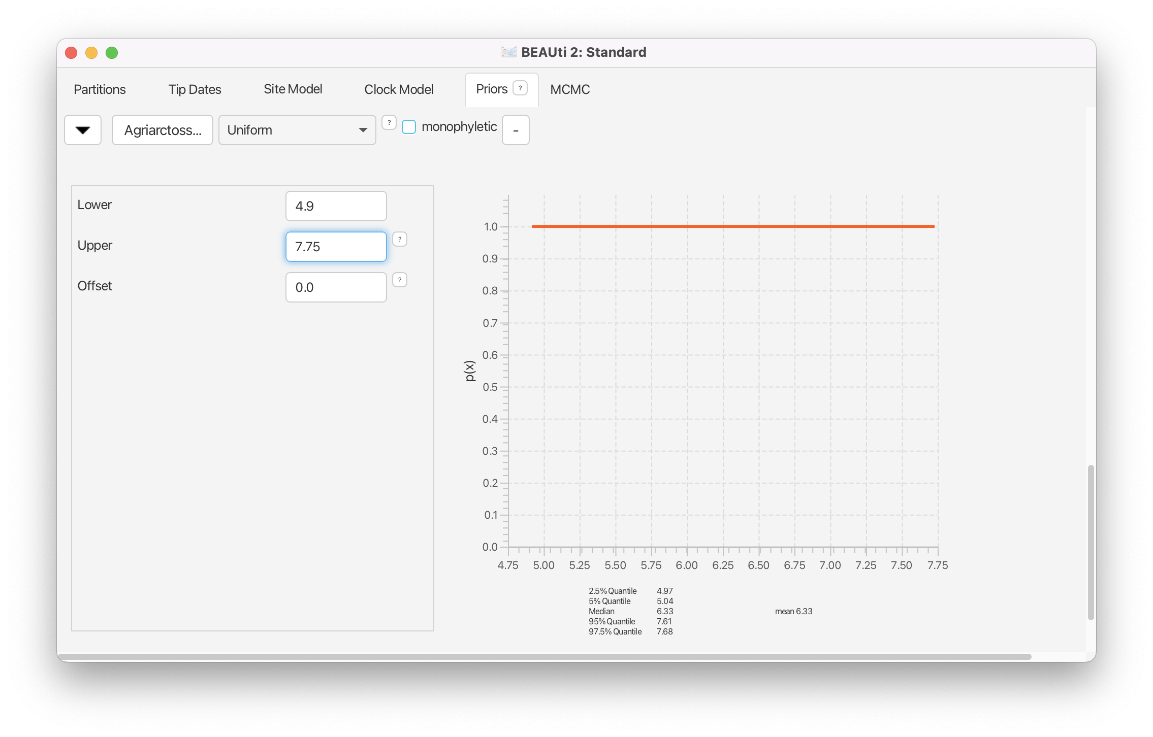
Back in the Priors window, reveal the options for the prior on the age of Agriarctos_spp by clicking on the $\blacktriangleright$. Change the prior distribution to Uniform, with a Lower value equal to 4.9 and an Upper value equal to 7.75. Check the box labeled Tipsonly.

Repeat for each of the 14 fossils in our dataset using the information in the table.

Set MCMC Options and Save the XML File

Now that you have specified all of your data elements, models, priors, and operators, go to the MCMC tab to set the length of the Markov chain, sample frequency, and file names.

Navigate to the MCMC window. Since we have a limited amount of time for this exercise, change the Chain Length to 2,000,000.

Reveal the options for the tracelog using the $\blacktriangleright$ to the left. Change Log Every to 100. Leave the name as the default.

Reveal the options for the treelog using the $\blacktriangleright$ to the left. Change Log Every to 100. Leave the name as the default.

Now we are ready to save the XML file!

In the pull-down menu save the file by going to File > Save As and save the file: bearsDivtime_FBD.xml.

For the last step in BEAUti, create an XML file that will run the analysis by sampling under the prior. This means that the MCMC will ignore the information coming from the sequence data and only sample parameters in proportion to their prior probability. The output files produced from this run will provide a way to visualize the marginal prior distributions on each parameter.

Check the box labeled Sample From Prior at the bottom of the MCMC panel.

Save these changes by going to File > Save As and name the file bearsDivtime_FBD.prior.xml.

Running BEAST 2

Now you are ready to start your BEAST analysis. BEAST allows you to use the BEAGLE library if you already have it installed. BEAGLE is an application programming interface and library that takes advantage of your computer hardware (CPUs and GPUs) for doing the heavy lifting (likelihood calculation) needed for statistical phylogenetic inference (Ayers et al., 2012). When using BEAGLE’s GPU (NVIDIA) implementation, runtimes are significantly shorter.

Execute bearsDivtime_FBD.prior.xml and bearsDivtime_FBD.xml in BEAST2. You should see the screen output every 1,000 generations, reporting the likelihood and several other statistics.

Summarizing the output

Once the run reaches the end of the chain, you will find three new files in your analysis directory. The MCMC samples of various scalar parameters and statistics are written to the file called bearsDivtime_FBD.log. The tree-state at every sampled iteration is saved to bearsDivtime_FBD-bearsTree.trees. The tree strings in this file are all annotated in extended Newick format with the substitution rate from the uncorrelated lognormal relaxed clock model at each node. The file called bearsDivtime_FBD.xml.state summarizes the performance of the proposal mechanisms (operators) used in your analysis, providing information about the acceptance rate for each move.

The main output files are the .log file and .trees files. We will use Tracer for assessing convergence, mixing, and determining an adequate burn-in based on the log file. Tree topologies, branch rates, and node heights are summarized using the program TreeAnnotator and visualized in FigTree.

Tracer

Provided with the files for this exercise are the output files from analyses run for 50,000,000 iterations. The files can be found under the Output heading in the left-hand column of this page and are all labeled with the file stem: bearsDivtime_FBD.*.log and bearsDivtime_FBD.*.trees. Note that the files are compressed with gzip (because they are quite large) and you’ll first need to extract them after downloading.

Open Tracer and import bearsDivtime_FBD.1.log, bearsDivtime_FBD.2.log and bearsDivtime_FBD.prior.log using File > Import New Trace File.

These log files are from two independent, identical analyses, and we can compare the log files in Tracer and determine if they have converged on the same stationary distribution. Additionally, analyzing samples from the prior allows you to compare your posterior estimates to the prior distributions used for each parameter.

Select and highlight all three files in the Trace Files pane (do not include Combined). This allows you to compare all three runs simultaneously. Click on the various parameters and view how they differ in their estimates and 95% credible intervals for those parameters.

The ORCsigma parameter indicates the amount of variation in the substitution rates across branches. Our prior on this parameter is an exponential distribution with $\nu = 2.997$ (mean $= 0.3337$). Thus, there is a considerable amount of prior weight on ORCsigma = 0. A standard deviation of 0 indicates support for no variation in substitution rates and the presence of a strict molecular clock.

Find the parameter ORCsigma and compare the estimates of the standard deviation of the uncorrelated log-normal distribution.

With ORCsigma highlighted for all three runs, go to the Marginal Density window, which allows you to compare the marginal posterior densities for each parameter. (By default Tracer gives the kernel density estimate (KDE) of the marginal density. You can change this to a Histogram using the options at the top of the window.)

Color the densities by Trace File next to Colour by at the bottom of the window (if you do not see this option, increase the size of your Tracer window). You can also add a Legend to reveal which density belongs to which run file.

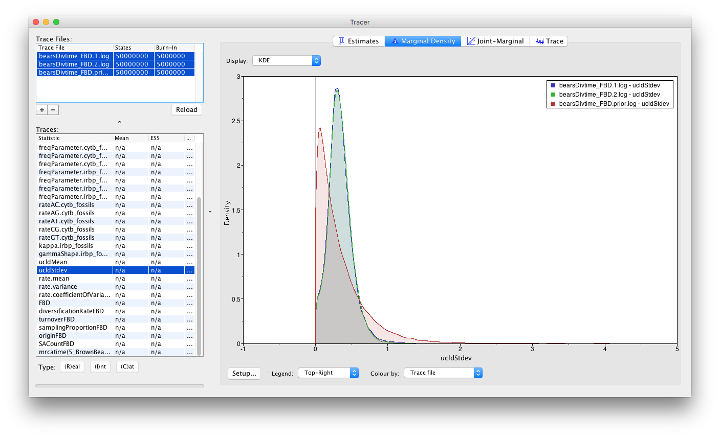
You will notice that the marginal densities from each of our analysis runs (bearsDivtime_FBD.1.log and bearsDivtime_FBD.2.log) are nearly identical. If you click through the other sampled parameters, these densities are the same for each one. This indicates that both of our runs have converged on the same stationary distribution. Also, it is likely that the ORC rates appear to be somewhat sensitive to the priors. That is because we have several lineages in our tree without any data, since we are using fossils to calibrate under the FBD model. For these branches, the clock rate assigned to them is sampled purely from the prior. The branches with extant descendants, however have rates that are informed by their DNA sequence data.

Next, we will look at the Marginal Distribution for the turnover parameter (turnoverFBD).

Select all trace files for the turnoverFBD parameter and go to the Marginal Density window. Color the densities by Trace file and add a legend.

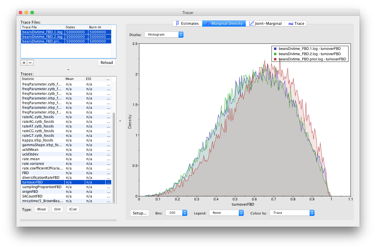
When comparing the MCMC with data to those sampled just under the prior, we can see that the prior and posterior densities are nearly identical. Additionally, you may be alarmed that the prior density looks nothing like the Uniform(0,1) prior we applied in BEAUti. However, it’s important to understand that when specifying Sample From Prior in BEAUti, we are telling BEAST to ignore the likelihood coming from the sequence data, but the MCMC continues to account for the other data—fossil occurrence times—that we have specified. Thus, since we have a good number of fossils, the estimates of turnover, diversification, and the sampling proportion are highly informed by these occurrence times.

Summarizing the Trees in Treeannotator

After reviewing the trace files from the two independent runs in Tracer and verifying that both runs converged on the posterior distributions and reached stationarity, we can combine the sampled trees into a single tree file and summarize the results.

Open the program LogCombiner and set the File type to Tree Files. Next, import bearsTree.1.trees and bearsTree.2.trees using the + button. Set a burn-in percentage of 20 for each file, thus discarding the first 20% of the samples in each tree file.

Both of these files contain 50,000 trees, so it is helpful to thin the tree samples and summarize fewer states to avoid creating unnecessarily large files.

Turn on Resample states at lower frequency and set this value to 10000.

Click on the Choose file … button to create an output file and run the program. Name the file: bearsTree.combined.trees.

Once LogCombiner has terminated, you will have a file containing 8,000 trees which can be summarized using TreeAnnotator. TreeAnnotator takes a collection of trees and summarizes them by identifying the topology with the best support, calculating clade posterior probabilities, and calculating 95% credible intervals for node-specific parameters. All of the node statistics are annotated on the tree topology for each node in the Newick string. We will generate a maximum clade credibility tree, which is the topology with the highest product of clade posterior probabilities across all nodes.

Open the program TreeAnnotator. Since we already discarded a set of burn-in trees when combining the tree files, we can leave Burnin set to 0 (though, if TreeAnnotator is taking a long time to load the trees, click on the Low memory option at the bottom left and set the burnin to 10–60% to reduce the number of trees). For the Target tree type, choose Maximum clade credibility tree. Choose Median heights for Node heights, and choose bearsTree.combined.trees as your Input Tree File. Then name the Output File bearsTree.summary.tre and click Run.

Visualizing the Dated Tree

The tree file produced by TreeAnnotator contains the maximum clade credibility tree and is annotated with summaries of the various parameters. The summary tree and it’s annotations can be visualized in the program FigTree.

Execute FigTree and open the file bearsTree.summary.tre.

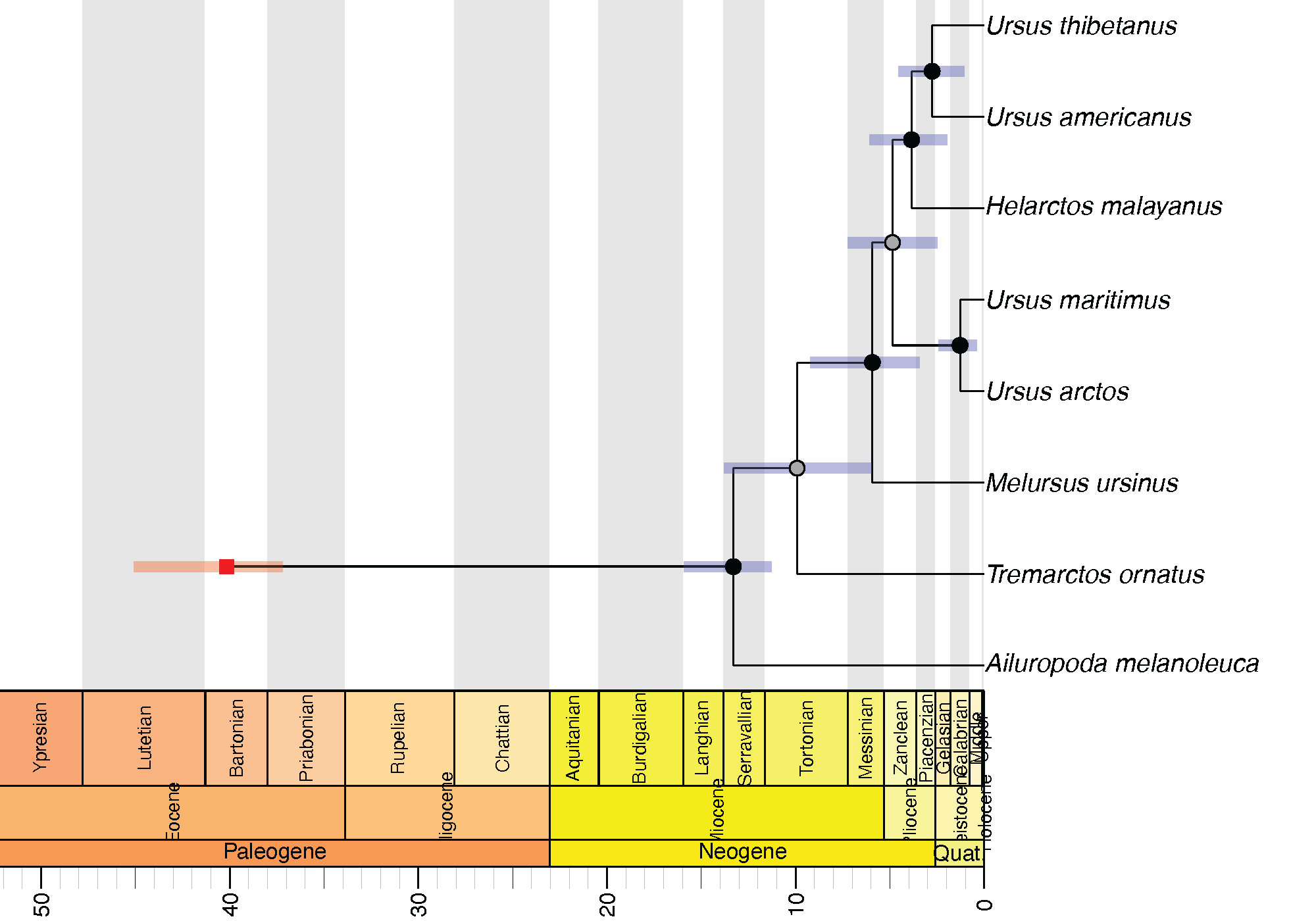
The tree you are viewing in FigTree has several fossil taxa with zero-length branches, e.g., Parictis montanus and Ursus abstrusus. These branches actually indicate fossil taxa with a significant probability of representing a sampled ancestor. However, it is difficult to represent this in typical tree-viewing programs. A tree with sampled ancestors properly represented will have two-degree nodes — i.e., a node with only one descendant. The web-based tree viewer IcyTree (Vaughan, 2017) is capable of plotting such trees from BEAST2 analyses.

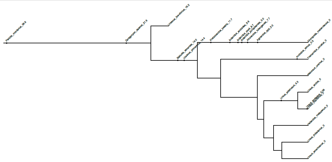
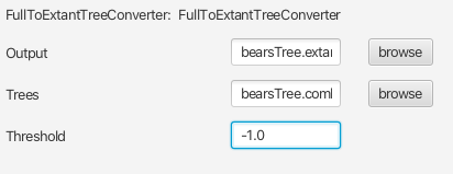
Although the tree above looks awesome, the topology can be misleading for this particular analysis. Because we did not provide character data for our 14 fossil taxa, the fossil lineages can attach to any lineage on the tree that is consistent with the monophyletic clades we specified and the fossil occurrence times with equal probability. However, we can prune off all of the fossil lineages, leaving only the tips infomed with DNA sequence data. We can do this using FullToExtantTreeConverter, then use TreeAnnotator to summarize the extant-only trees.

Open BEAUti and launch the accessory apps via File > Launch Apps. This will open a window with a few applications, launch FullToExtantTreeConverter. In the file specification window for Trees provide the file called bearsTree.combined.trees. And give the Output file the name bearsTree.extant.trees.

Run TreeAnnotator on the file called bearsTree.extant.trees, selecting the same options as you did for the file with complete trees. Name the summary tree file bearsTree.extant_summary.tre.

R code is also provided in the Scripts directory, which can be used to plot the tree against a geological timescale using the strap package (Bell & Lloyd, 2014).

Useful Links

• Bayesian Evolutionary Analysis with BEAST 2 (Drummond & Bouckaert, 2014)
• BEAST 2 website and documentation: http://www.beast2.org/
• BEAST 1 website and documentation: http://beast.bio.ed.ac.uk
• RevBayes: https://github.com/revbayes/code
• DPPDiv: https://github.com/trayc7/FDPPDIV
• PhyloBayes: www.phylobayes.org/
• multidivtime: http://statgen.ncsu.edu/thorne/multidivtime.html
• MCMCTree (PAML): http://abacus.gene.ucl.ac.uk/software/paml.html
• BEAGLE: https://github.com/beagle-dev/beagle-lib
• Paleobiology Database: http://www.paleodb.org
• Fossil Calibration Database: http://fossilcalibrations.org
• Join the BEAST user discussion: http://groups.google.com/group/beast-users

Relevant References

1. Drummond, A. J., Ho, S. Y., Phillips, M. J., & Rambaut, A. (2006). Relaxed phylogenetics and dating with confidence. PLoS Biology, 4, e88.
2. Drummond, A. J., & Rambaut, A. (2007). BEAST: Bayesian evolutionary analysis by sampling trees. BMC Evolutionary Biology, 7, 214.
3. Bouckaert, R., Heled, J., Kühnert, D., Vaughan, T., Wu, C.-H., Xie, D., Suchard, M. A., Rambaut, A., & Drummond, A. J. (2014). BEAST 2: A Software Platform for Bayesian Evolutionary Analysis. PLoS Computational Biology, 10(4), e1003537.
4. Krause, J., Unger, T., Noçon, A., Malaspinas, A.-S., Kolokotronis, S.-O., Stiller, M., Soibelzon, L., Spriggs, H., Dear, P. H., Briggs, A. W., & others. (2008). Mitochondrial genomes reveal an explosive radiation of extinct and extant bears near the Miocene-Pliocene boundary. BMC Evolutionary Biology, 8(1), 220.
5. dos Reis, M., Inoue, J., Hasegawa, M., Asher, R. J., Donoghue, P. C. J., & Yang, Z. (2012). Phylogenomic datasets provide both precision and accuracy in estimating the timescale of placental mammal phylogeny. Proceedings of the Royal Society B: Biological Sciences, 279(1742), 3491–3500.
6. Stadler, T. (2010). Sampling-through-time in birth-death trees. Journal of Theoretical Biology, 267, 396–404.
7. Heath, T. A., Huelsenbeck, J. P., & Stadler, T. (2014). The fossilized birth-death process for coherent calibration of divergence-time estimates. Proceedings of the National Academy of Sciences, USA, 111, E2957–E2966.
8. Gavryushkina, A., Welch, D., Stadler, T., & Drummond, A. J. (2014). Bayesian inference of sampled ancestor trees for epidemiology and fossil calibration. PLoS Computational Biology, 10(12), e1003919.
9. Clark, J., & Guensburg, T. E. (1972). Arctoid Genetic Characters as Related to the Genus \emphParictis (Vol. 1150). Field Museum of Natural History.
10. Ginsburg, L., & Morales, J. (1995). \textitZaragocyon daamsi n. gen. sp. nov., Ursidae primitif du Miocène inférieur d’Espagne. Comptes Rendus De l’Académie Des Sciences. Série 2. Sciences De La Terre Et Des Planètes, 321(9), 811–815.
11. Abella, J., Alba, D. M., Robles, J. M., Valenciano, A., Rotgers, C., Carmona, R., Montoya, P., & Morales, J. (2012). \textitKretzoiarctos gen. nov., the Oldest Member of the Giant Panda Clade. PLoS One, 17, e48985.
12. Ginsburg, L., & Morales, J. (1998). Les Hemicyoninae (Ursidae, Carnivora, Mammalia) et les formes apparentées du Miocène inférieur et moyen d’Europe occidentale. Annales De Paléontologie, 84(1), 71–123.
13. Andrews, P., & Tobien, H. (1977). New Miocene locality in Turkey with evidence on the origin of \textitRamapithecus and \textitSivapithecus. Nature, 268(5622), 699.
14. Heizmann, E., Ginsburg, L., & Bulot, C. (1980). \textitProsansanosmilus peregrinus, ein neuer machairodontider Felidae aus dem Miozän Deutschlands und Frankreichs. Stuttgarter Beitr. Naturk. B, 58, 1–27.
15. Montoya, P., Alcalá, L., & Morales, J. (2001). \textitIndarctos (Ursidae, Mammalia) from the Spanish Turolian (Upper Miocene). Scripta Geologica, 122, 123–151.
16. Geraads, D., Kaya, T., Mayda, S., & others. (2005). Late Miocene large mammals from Yulafli, Thrace region, Turkey, and their biogeographic implications. Acta Palaeontologica Polonica, 50(3), 523–544.
17. Baryshnikov, G. F. (2002). Late Miocene \textitIndarctos punjabiensis atticus (Carnivora, Ursidae) in Ukraine with survey of \textitIndarctos records from the former USSR. Russian J. Theriol, 1(2), 83–89.
18. Jin, C., Ciochon, R. L., Dong, W., Hunt, R. M., Liu, J., Jaeger, M., & Zhu, Q. (2007). The first skull of the earliest giant panda. Proceedings of the National Academy of Sciences, 104(26), 10932–10937.
19. Abella, J., Montoya, P., & Morales, J. (2011). Una nueva especie de \textitAgriarctos (Ailuropodinae, Ursidae, Carnivora) en la localidad de Nombrevilla 2 (Zaragoza, España). Estudios Geológicos, 67(2), 187–191.
20. Churcher, C. S., Morgan, A. V., & Carter, L. D. (1993). \textitArctodus simus from the Alaskan Arctic slope. Canadian Journal of Earth Sciences, 30(5), 1007–1013.
21. Bjork, P. R. (1970). The Carnivora of the Hagerman local fauna (late Pliocene) of Southwestern Idaho. Transactions of the American Philosophical Society, 60(7), 3–54.
22. Loreille, O., Orlando, L., Patou-Mathis, M., Philippe, M., Taberlet, P., & Hänni, C. (2001). Ancient DNA analysis reveals divergence of the cave bear, \textitUrsus spelaeus, and brown bear, \textitUrsus arctos, lineages. Current Biology, 11(3), 200–203.
23. Ayers, D. L., Darling, A., Zwickl, D. J., Beerli, P., Holder, M. T., Lewis, P. O., Huelsenbeck, J. P., Ronquist, F., Swofford, D. L., Cummings, M. P., Rambaut, A., & Suchard, M. A. (2012). BEAGLE: An Application Programming Interface and High-Performance Computing Library for Statistical Phylogenetics. Systematic Biology, 61, 170–173.
24. Vaughan, T. G. (2017). IcyTree: Rapid browser-based visualization for phylogenetic trees and networks. Bioinformatics, in press. https://doi.org/https://doi.org/10.1093/bioinformatics/btx155
25. Bell, M. A., & Lloyd, G. T. (2014). strap: an R package for plotting phylogenies against stratigraphy and assessing their stratigraphic congruence. Palaeontology.
26. Drummond, A. J., & Bouckaert, R. R. (2014). Bayesian evolutionary analysis with BEAST 2. Cambridge University Press.

---

Citation

If you found Taming the BEAST helpful in designing your research, please cite the following paper:

Joëlle Barido-Sottani, Veronika Bošková, Louis du Plessis, Denise Kühnert, Carsten Magnus, Venelin Mitov, Nicola F. Müller, Jūlija Pečerska, David A. Rasmussen, Chi Zhang, Alexei J. Drummond, Tracy A. Heath, Oliver G. Pybus, Timothy G. Vaughan, Tanja Stadler (2018). Taming the BEAST – A community teaching material resource for BEAST 2. Systematic Biology, 67(1), 170–-174. doi: 10.1093/sysbio/syx060