


Background
In Bayesian divergence-time estimation, phylogenies are commonly time calibrated through the specification of calibration densities on nodes that represent clades with known fossil occurrences. Unfortunately, the optimal shape of these calibration densities is usually unknown and they are therefore often chosen arbitrarily, which directly impacts the reliability of the resulting age estimates. CladeAge overcomes this limitation by calculating optimal calibration densities for clades with fossil records, based on estimates for diversification rates and the sampling rate for fossils. CladeAge thus shares similarities with the Fossilized Birth-Death (FBD) process; however, while the FBD model assumes that the fossil record is either completely or randomly sampled, the CladeAge model assumes that only information about the oldest fossil of each clade is available and can provide unbiased age estimates in such cases. CladeAge allows uncertainty in the diversification- and sampling-rate estimates, but unlike with the FBD model, these parameters must be known a priori and can not be estimated as part of the analysis.
Programs Used in This Tutorial
BEAST2 - Bayesian Evolutionary Analysis Sampling Trees 2
BEAST2 is a free software package for Bayesian evolutionary analysis of molecular sequences using MCMC and strictly oriented toward inference using rooted, time-measured phylogenetic trees (Bouckaert et al., 2014). This tutorial uses the BEAST2 version 2.5.0.
BEAUti2 - Bayesian Evolutionary Analysis Utility
BEAUti2 is a graphical user interface tool for generating BEAST2 XML configuration files.
Both BEAST2 and BEAUti2 are Java programs, which means that the exact same code runs on all platforms. For us it simply means that the interface will be the same on all platforms. The screenshots used in this tutorial are taken on a Mac OS X computer; however, both programs will have the same layout and functionality on both Windows and Linux. BEAUti2 is provided as a part of the BEAST2 package so you do not need to install it separately.
Tracer
Tracer (http://tree.bio.ed.ac.uk/software/tracer) is used to summarize the posterior estimates of the various parameters sampled by the Markov Chain. This program can be used for visual inspection and to assess convergence. It helps to quickly view median estimates and 95% highest posterior density intervals of the parameters, and calculates the effective sample sizes (ESS) of parameters. It can also be used to investigate potential parameter correlations. We will be using Tracer v1.6.0.
TreeAnnotator
TreeAnnotator is used to summarize the posterior sample of trees to produce a maximum-clade-credibility tree. It can also be used to summarize and visualize the posterior estimates of other tree parameters (e.g. node height). TreeAnnotator is provided as a part of the BEAST2 package so you do not need to install it separately.
FigTree
FigTree (http://tree.bio.ed.ac.uk/software/figtree) is a program for viewing trees and producing publication-quality figures. It can interpret the node annotations created on the summary trees by TreeAnnotator, allowing the user to display node-based statistics (e.g. posterior probabilities). We will be using FigTree v1.4.2.
Tutorial: Fossil-Based Divergence-Time Estimation With CladeAge
In this tutorial, we are going to use a multi-marker sequence dataset in combination with fossil information to estimate the divergence times of cichlid fishes with the CladeAge model.
The aim of this tutorial is to:
- Learn which fossil information is required to apply the CladeAge model.
- Learn how to estimate divergence times with CladeAge.
The data
The analyses in this tutorial will be based on the dataset of Near et al. (“Phylogeny and Tempo of Diversification in the Superradiation of Spiny-Rayed Fishes,” 2013), comprising alignments for ten nuclear genes. In their study, Near et al. (“Phylogeny and Tempo of Diversification in the Superradiation of Spiny-Rayed Fishes,” 2013) used this dataset to estimate divergence times of spiny-rayed fishes (=Acanthomorphata), and to identify shifts in diversification rates among different groups of these fishes. While the dataset of Near et al. (“Phylogeny and Tempo of Diversification in the Superradiation of Spiny-Rayed Fishes,” 2013) did not focus on cichlid diversification, it included nine cichlid species among the 608 species sampled for the extensive phylogeny. Thus, we can here use part of this dataset of Near et al. (“Phylogeny and Tempo of Diversification in the Superradiation of Spiny-Rayed Fishes,” 2013) to estimate early divergences among cichlid fishes. To facilitate the analyses in this tutorial, we will reduce the dataset of Near et al. (“Phylogeny and Tempo of Diversification in the Superradiation of Spiny-Rayed Fishes,” 2013) to sequences of 24 selected species. These species represent divergent cichlid lineages as well as the most ancestral groups of spiny-rayed fishes so that the fossil record of these lineages can be employed for calibration.
The CladeAge model
The approach of CladeAge is similar to the more traditional node-dating approach in the sense that prior densities are defined for the ages of different clades, and the minimum ages of these prior densities are provided by the oldest fossils of these clades. However, important differences exist between the CladeAge approach and node dating: First, the shape of age-prior densities is informed by a model of diversification and fossil sampling in the CladeAge approach, whereas in node dating, parametric distributions (e.g. lognormal or gamma) with more or less arbitrarily chosen parameters are usually applied. Second, because of the quantitative model used in the CladeAge approach, the clades used for calibration should also not be chosen at will. Instead, strictly all clades included in the phylogeny that (i) have a fossil record, (ii) are morphologically recognizable, and (iii) have their sister lineage also included in the phylogeny should be constrained according to the age of their oldest fossil. A consequence of this is that clades are constrained even when their known sister lineage has an older fossil record, and that the same fossil may be used to constrain not just one clade, but multiple nested clades, if the more inclusive clades do not have an even older fossil record. More details about these criteria can be found in our paper on CladeAge (Matschiner et al., 2017), and further information on using CladeAge is given in our Rough Guide to CladeAge.
Divergence-time estimation with CladeAge
Preparing the molecular dataset
As a first step, download the molecular dataset of Near et al. (“Phylogeny and Tempo of Diversification in the Superradiation of Spiny-Rayed Fishes,” 2013) from the Dryad data repository connected to their publication. On the command-line of a Mac or Linux computer, this could be done using the wget utility.
Execute the following command:
wget https://datadryad.org/bitstream/handle/10255/dryad.50839/Near_et_al.nex
Alternatively, you could use your browser to open the Dryad repository https://datadryad.org/resource/doi:10.5061/dryad.d3mb4 and download the file Near_et_al.nex.
This file in Nexus format contains the sequence alignments for ten nuclear markers, sequenced for 608 species of spiny-rayed fishes. As this dataset is far too large to be analyzed in this tutorial, we’ll extract the sequences of 24 species that represent major groups of spiny-rayed fishes (Betancur-R et al., 2017) as well as the most divergent groups of cichlid fishes. The 24 species that we will focus on are listed in the table below.
A list of the 24 species IDs in plain text format is also in file Near_et_al_ids.txt. On the command line, we can use that file to extract the sequences of these species from the full alignment, and write them to a new file in Nexus format named Near_et_al_red.nex.
Execute the following commands on the command line, after placing file
Near_et_al_ids.txtin the same directory asNear_et_al.nex:
head -n 7 Near_et_al.nex | sed 's/ntax=608/ntax=24/g'> Near_et_al_red.nex
grep -f Near_et_al_ids.txt -e "\[" Near_et_al.nex | sed -e $'s/\[/\\\n\[/g' >> Near_et_al_red.nex
tail -n 35 Near_et_al.nex | sed 's/paup/assumptions/g' >> Near_et_al_red.nex
If you should not be able to execute these commands on the command line, you could instead download the reduced alignment file Near_et_al_red.nex using the link in the left-hand menu under “Data”.
Installing the CladeAge package
To use fossil constraints as calibrations points according to the CladeAge model, we’ll first have to install the CladeAge add-on package for BEAST2.
To do so, open BEAUti, and click on “Manage Packages” in the “File” menu.
This will open a window for the BEAST2 Package Manager. In this window, select “CA” and click “Install/Upgrade” as shown in the screenshot below.
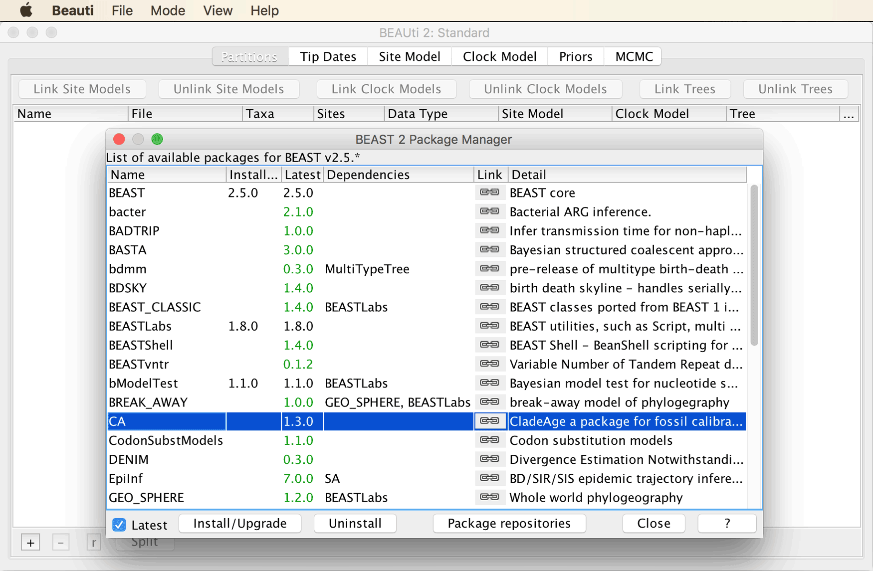
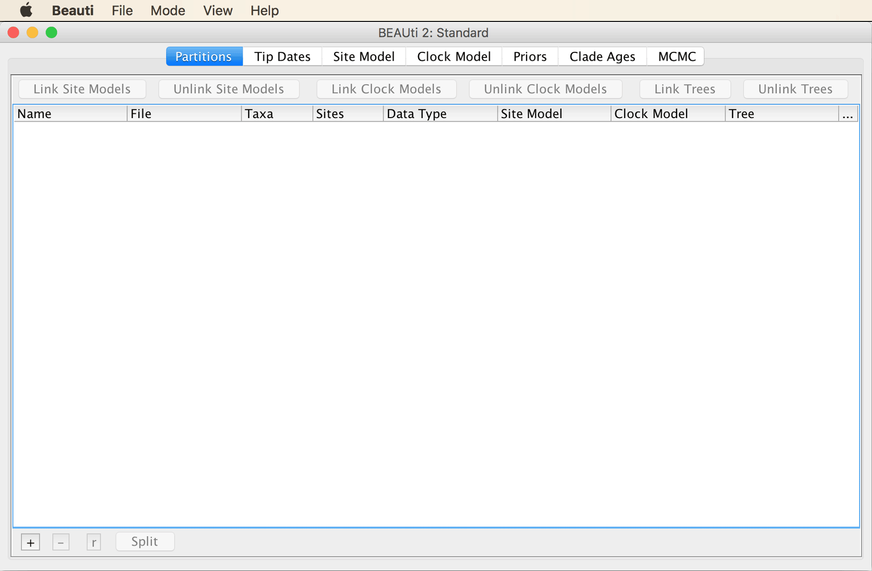
Close and reopen BEAUti.
You should then see that an additional tab has been added named “Clade Ages”, as in the screenshot below.
Generating the analysis file with BEAUti
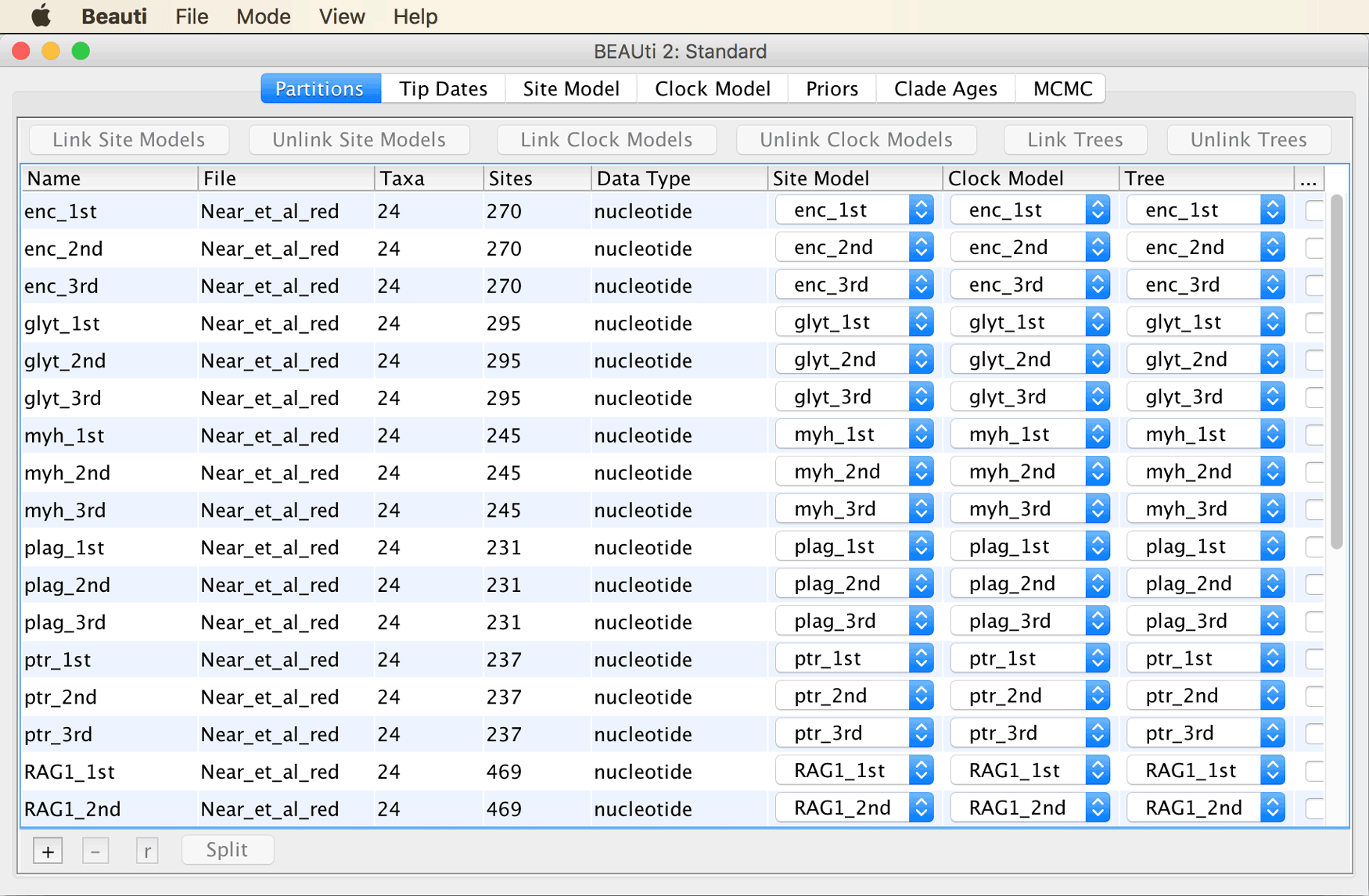
Click on “Import Alignment” in BEAUti’s “File” menu, and select the alignment file
Near_et_al_red.nex.
BEAUti should recognize 30 different partitions, one for each codon position of each of the ten markers. The BEAUti window should then look as shown in the screenshot below.
Select all partitions, and click “Link Trees” as well as “Link Clock Models”, as shown below.
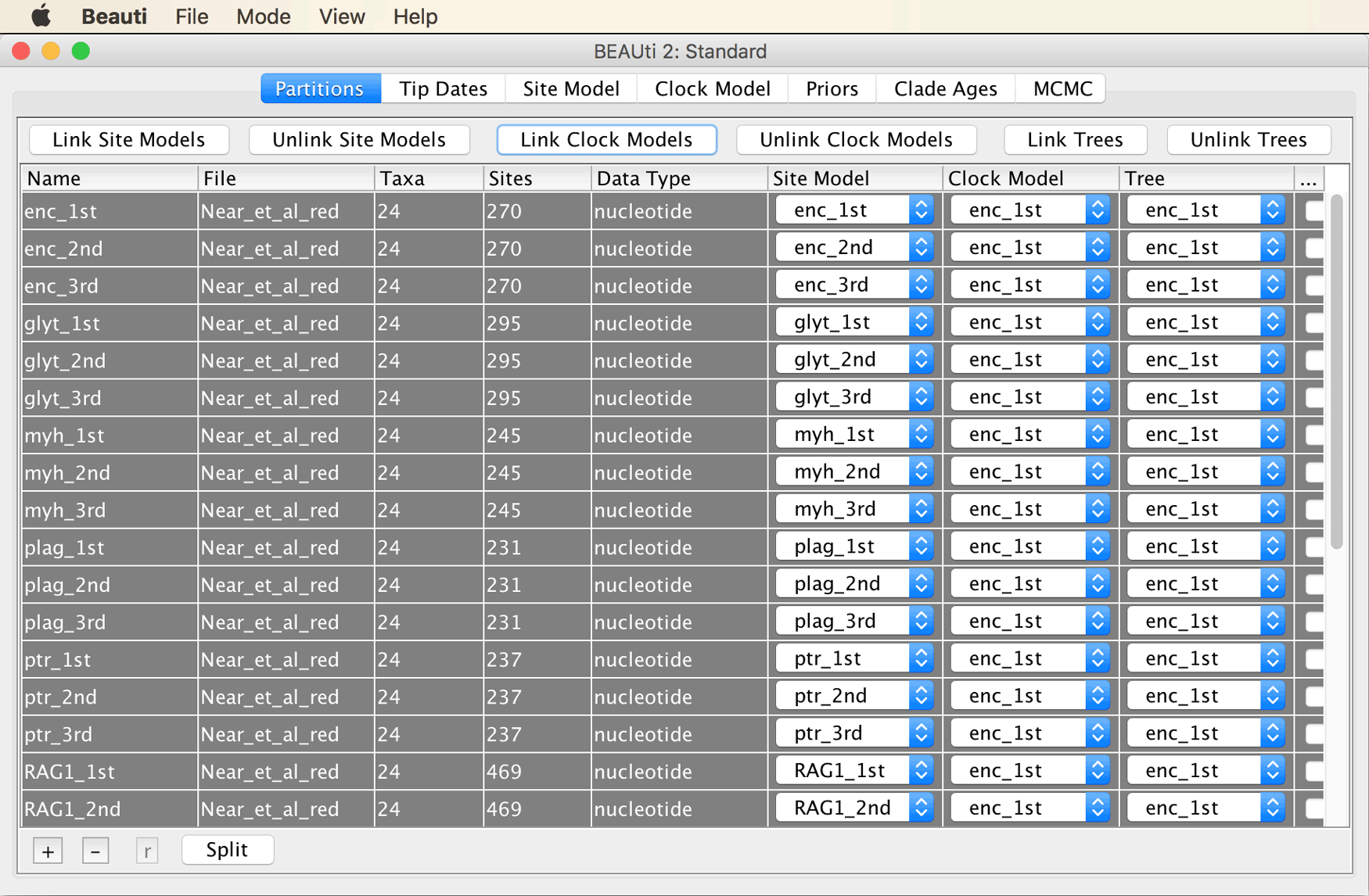
Move on to the “Site Model” tab to select the site model for all partitions.
Instead of selecting a model such as HKY or GTR, I highly recommend the use of the model-averaging approach implemented in the bModelTest package (Bouckaert & Drummond, 2017). If you did not already install this package, you can do so with the BEAST2 Package Manager from BEAUti as described above for the installation of the CladeAge package (don’t forget to close and reopen BEAUti after installation to see changes to the interface). More information on model averaging with the bModelTest package is provided in the Substitution Model Averaging tutorial. While recommended, model averaging with bModelTest is not required for this CladeAge tutorial, and you could also pick a model such as HKY or GTR instead. The description given here, however, assumes that the bModelTest package has been installed.
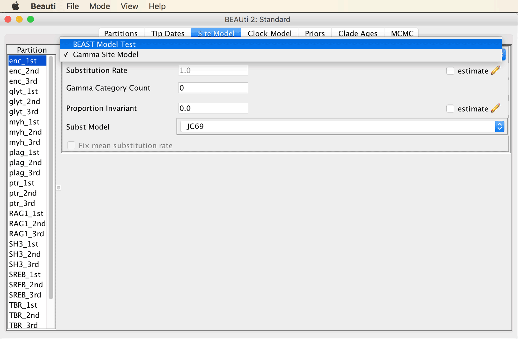
Select “BEAST Model Test” from the drop-down menu at the top of the window, as shown below.
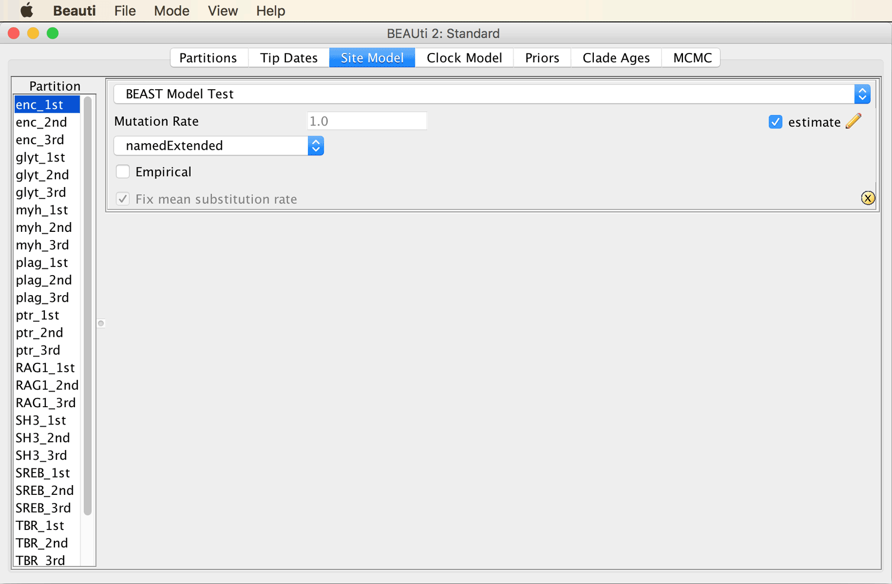
Select “namedExtended” from the drop-down menu that at first had “transitionTransversionSplit” selected. Leave the checkbox next to “Empirical” unticked to allow estimation of nucleotide frequencies. Then, set the tick to the right of “Mutation Rate” to specify that this rate should be estimated.
The window should then look as in the next screenshot.
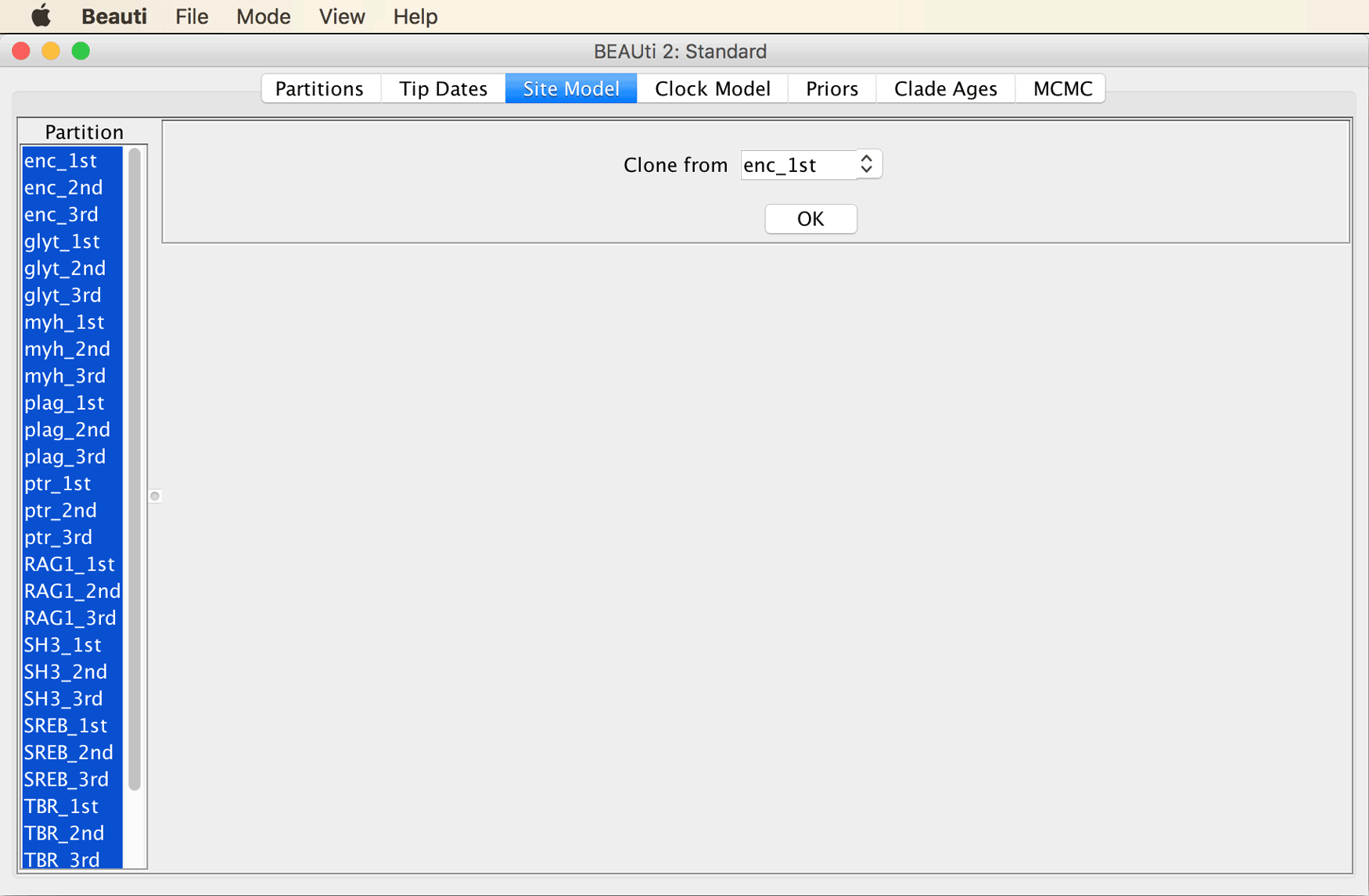
Select all partitions in the list at the left of the window, and click “OK” to clone the site model from the first partition to all other partitions.
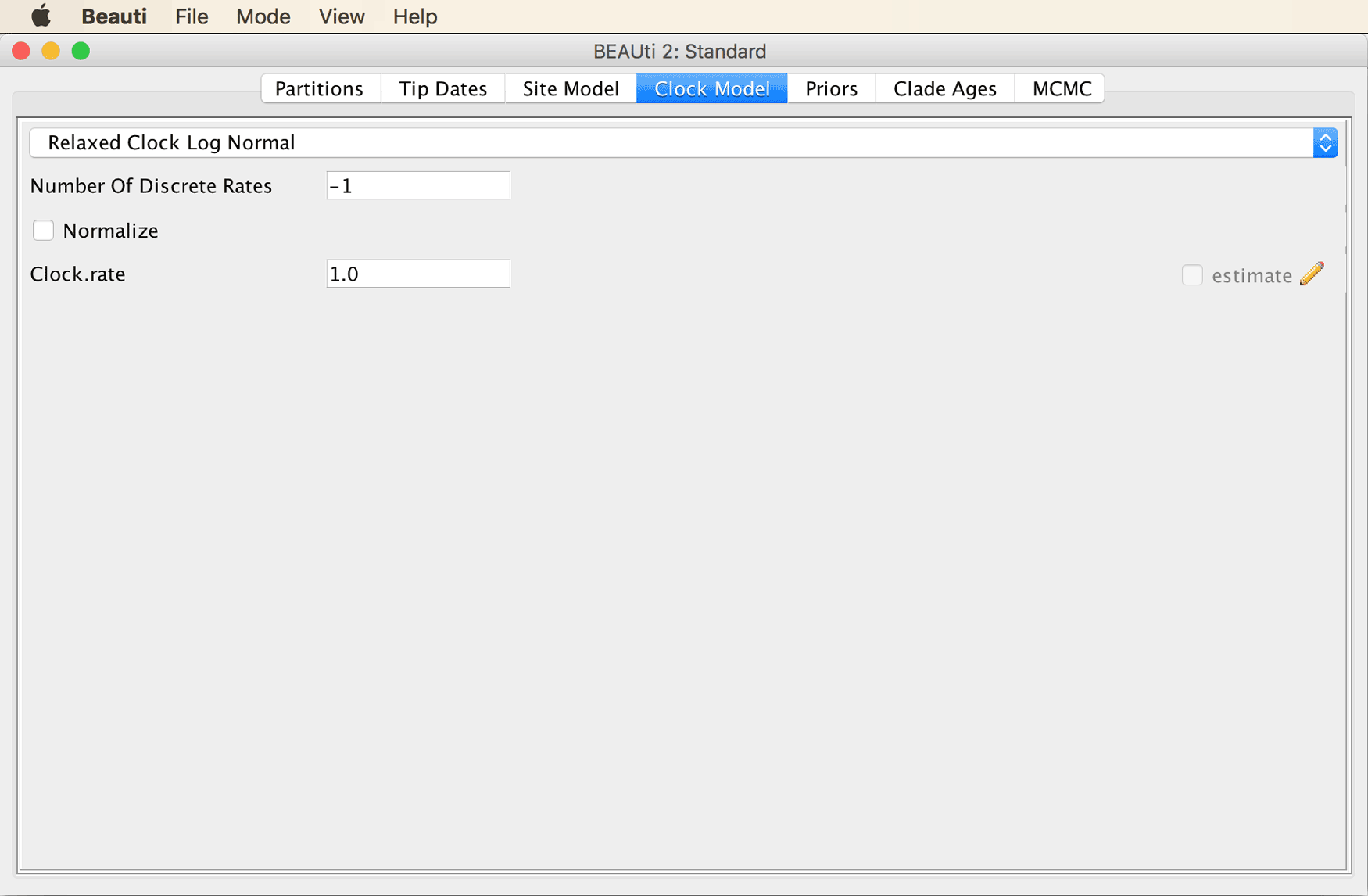
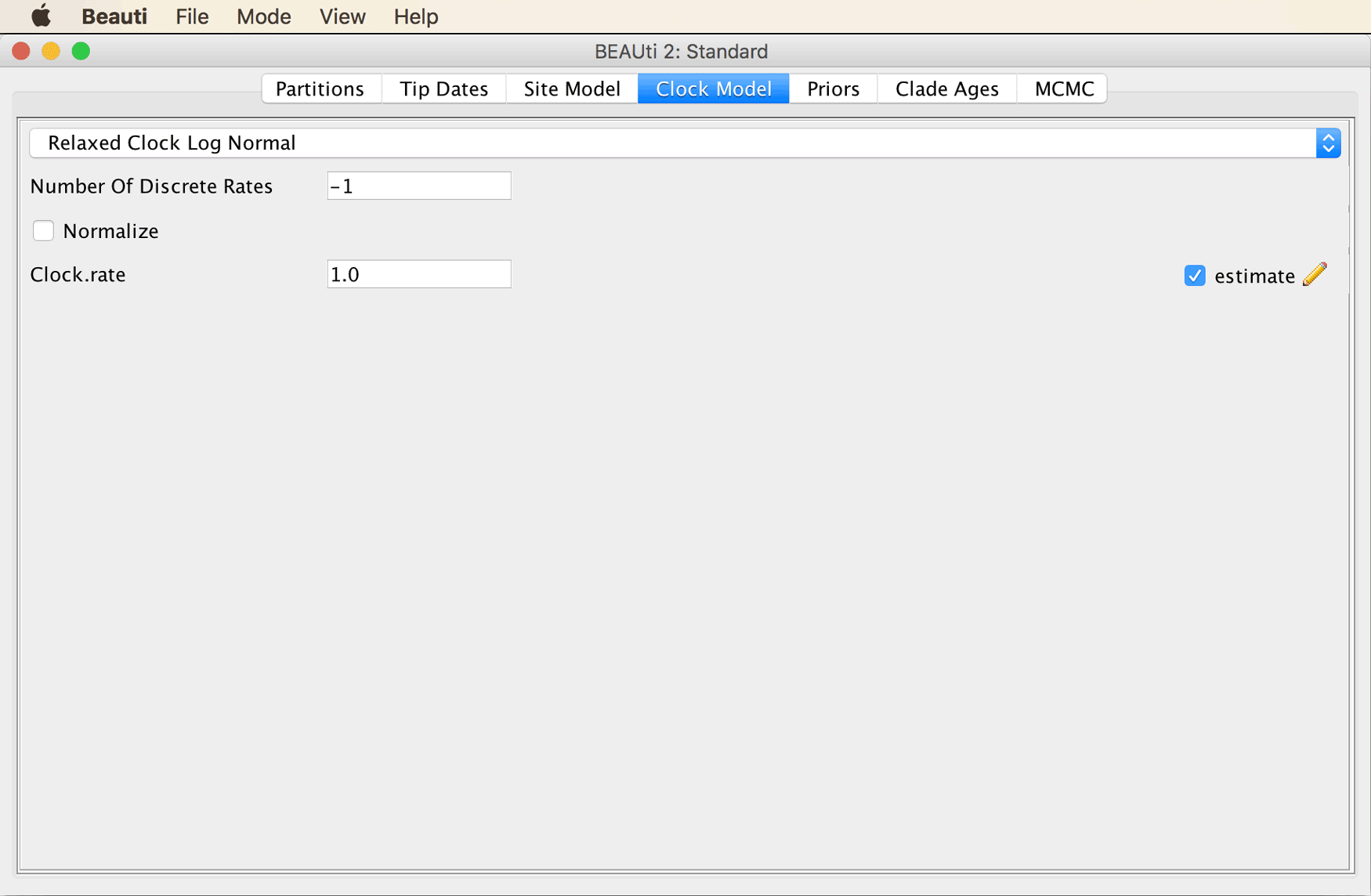
Continue to the “Clock Model” tab, and select the “Relaxed Clock Log Normal” clock model from the drop-down menu.
Because we are going to calibrate the molecular clock with fossil constraints, we should allow the clock rate to be estimated. By default, however, the checkbox that we would need to tick, next to “estimate” at the bottom right, is disabled.
To enable this checkbox, click on “Automatic set clock rate” in BEAUti’s “Mode” menu.
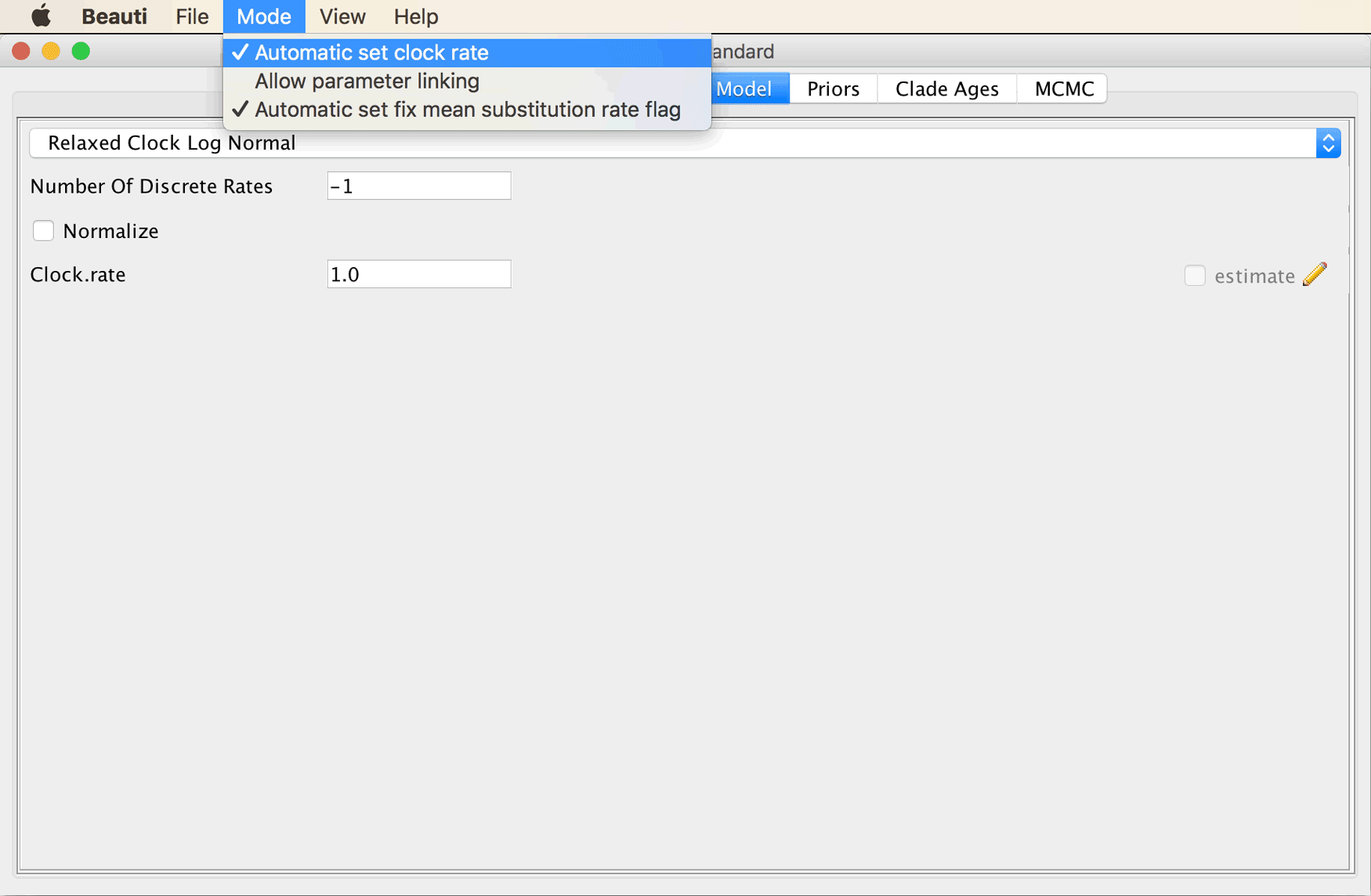
The checkbox for clock-rate estimation should then be enabled.
Set a tick in the checkbox at the bottom right to estimate the clock rate.
The “Clock Model” tab should then look as shown in the screenshot below.
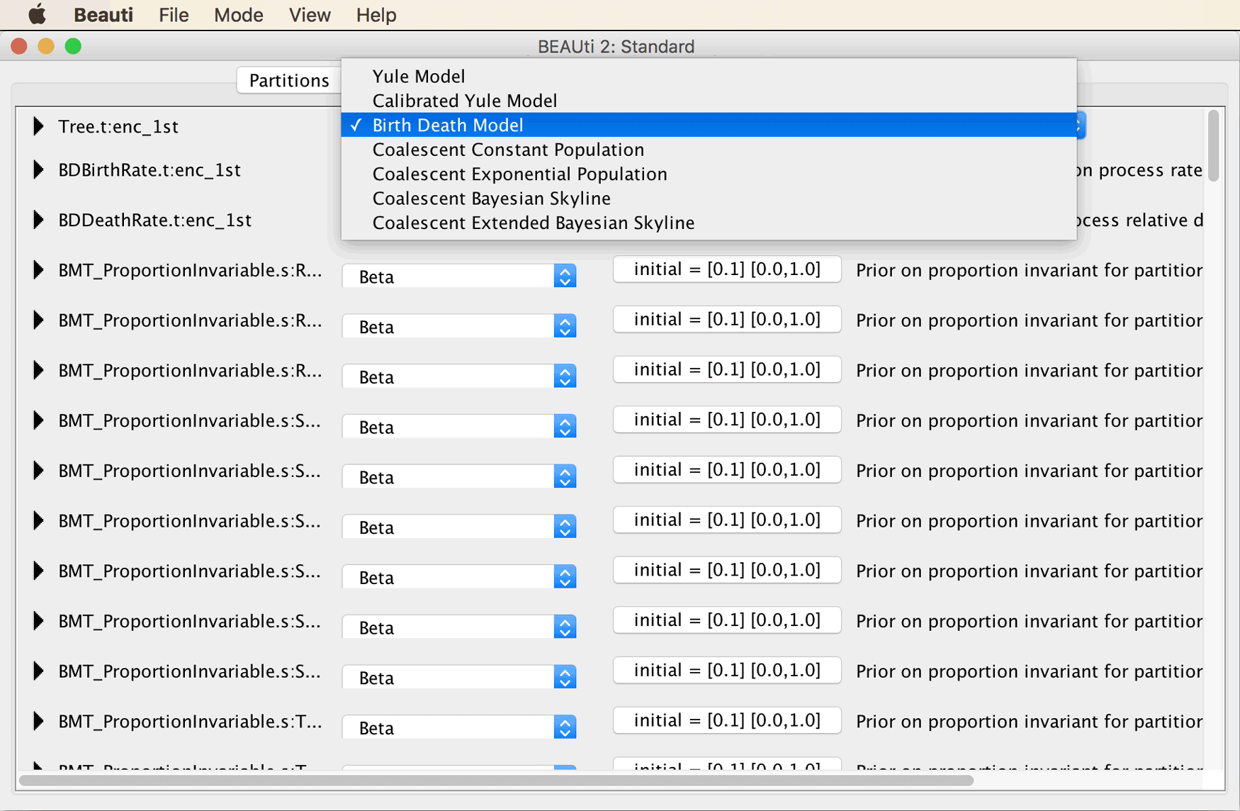
Move on to the “Priors” tab. Select the “Birth Death Model” as the tree prior, from the drop-down menu at the very top of the window.
Instead of specifying constraints on monophyly and divergence times in the “Priors” tab (as is usually the case), this is done in the separate tab named “Clade Ages” when the CladeAge package is installed.
Open the “Clade Ages” tab and click on the “+ Add Prior” button
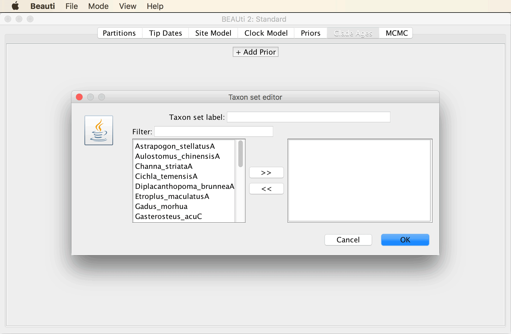
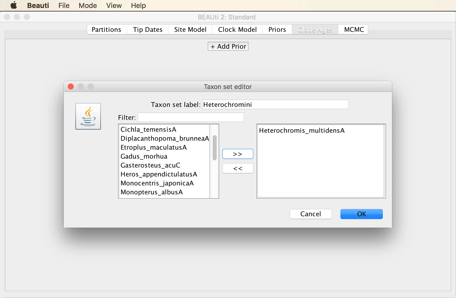
We will now have to specify a rather long list of constraints to make the best possible use of the information provided by the fossil record and to obtain divergence time estimates that are as reliable as possible given our dataset. We’ll start simple by specifying that the origin of African cichlid tribe Heterochromini, represented in our dataset by Heterochromis multidens, must have occurred at least 15.97-33.9 million years ago (Ma), since this is the age of the oldest fossil of Heterochromi, which was reported from the Baid Formation of Saudi Arabia by Lippitsch and Micklich (“Cichlid Fish Biodiversity in an Oligocene Lake,” 1998).
Specify “Heterochromini” in the field next to “Taxon set label”, and select only “Heterochromis_multidensA” as the ingroup of this taxon set.
After you click “OK”, you’ll see the window shown below, in which you can specify minimum and maximum values for the parameters net diversification rate, turnover rate, and sampling rate. Based on these values as well as the fossil age, the CladeAge model is going to automatically determine the optimal shape of the prior density used for each constraint.
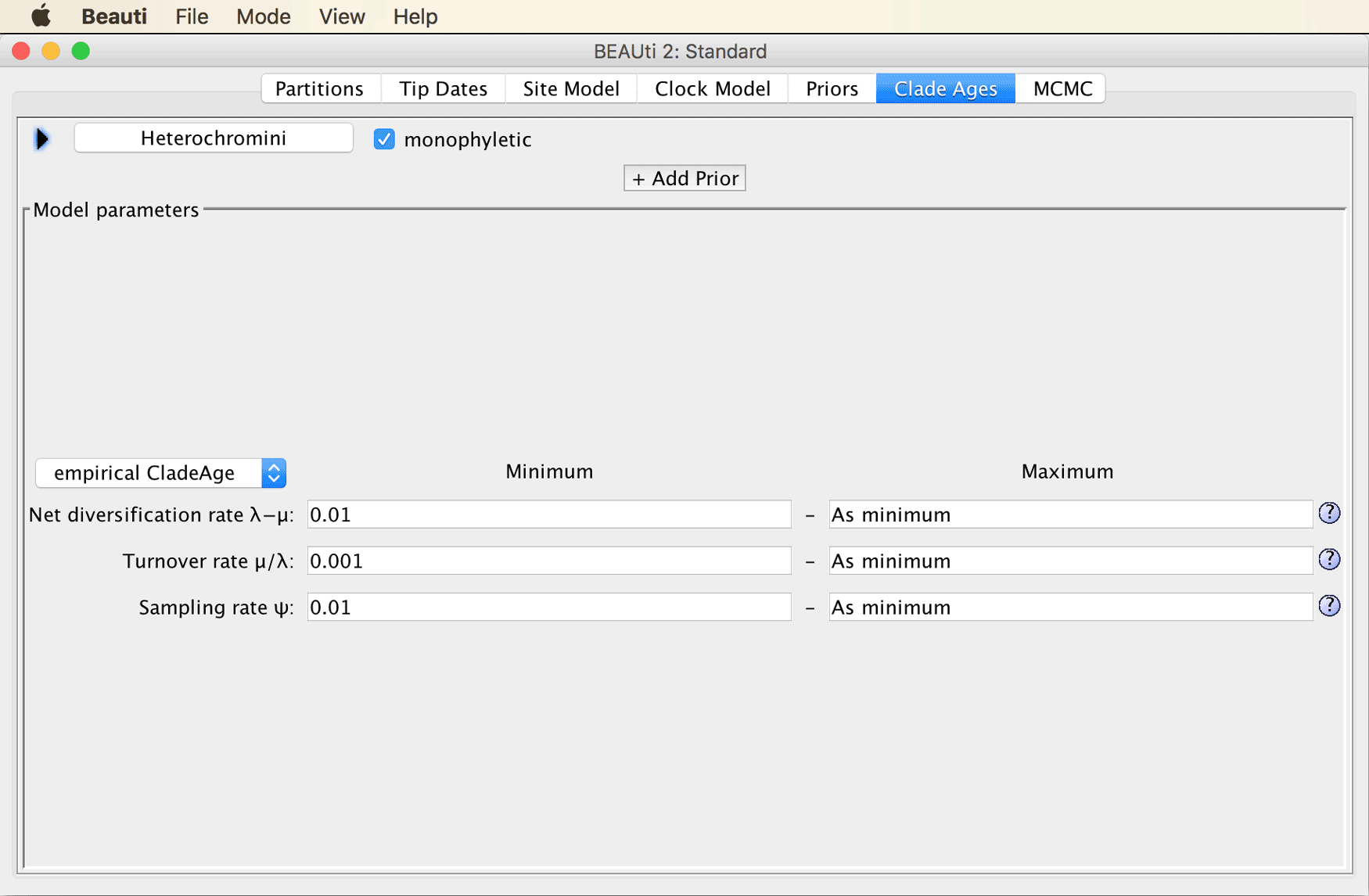
While it might sometimes be preferable to estimate the net diversification (speciation minus extinction) and turnover (extinction divided by speciation) rates as part of the analysis, this is not implemented in the CladeAge model yet. Instead, the values for the two parameters have to be specified a priori, together with the “sampling rate”, the rate at which fossils that are eventually sampled by scientists were once deposited in the fossil record. Fortunately, estimates for these three rates can be found in the literature, and the confidence intervals for these estimates can be accounted for by the CladeAge model. Here, as in Matschiner et al. (“Bayesian Phylogenetic Estimation of Clade Ages Supports Trans-Atlantic Dispersal of Cichlid Fishes,” 2017), we adopt teleost-specific estimates for net diversification and turnover from Santini et al. (“Did Genome Duplication Drive the Origin of Teleosts? A Comparative Study of Diversification in Ray-Finned Fishes,” 2009), and a sampling-rate estimate for bony fishes from Foote and Miller (Principles of Paleontology, 2007). These estimates are 0.041-0.081 for the net diversification rate, 0.0011-0.37 for the turnover, and 0.0066-0.01806 for the sampling rate.
Specify 0.041-0.081 for the net diversification rate, 0.0011-0.37 for the turnover, and 0.0066-0.01806 for the sampling rate. Don’t change the selection of “empirical CladeAge” in the drop-down menu to the left.
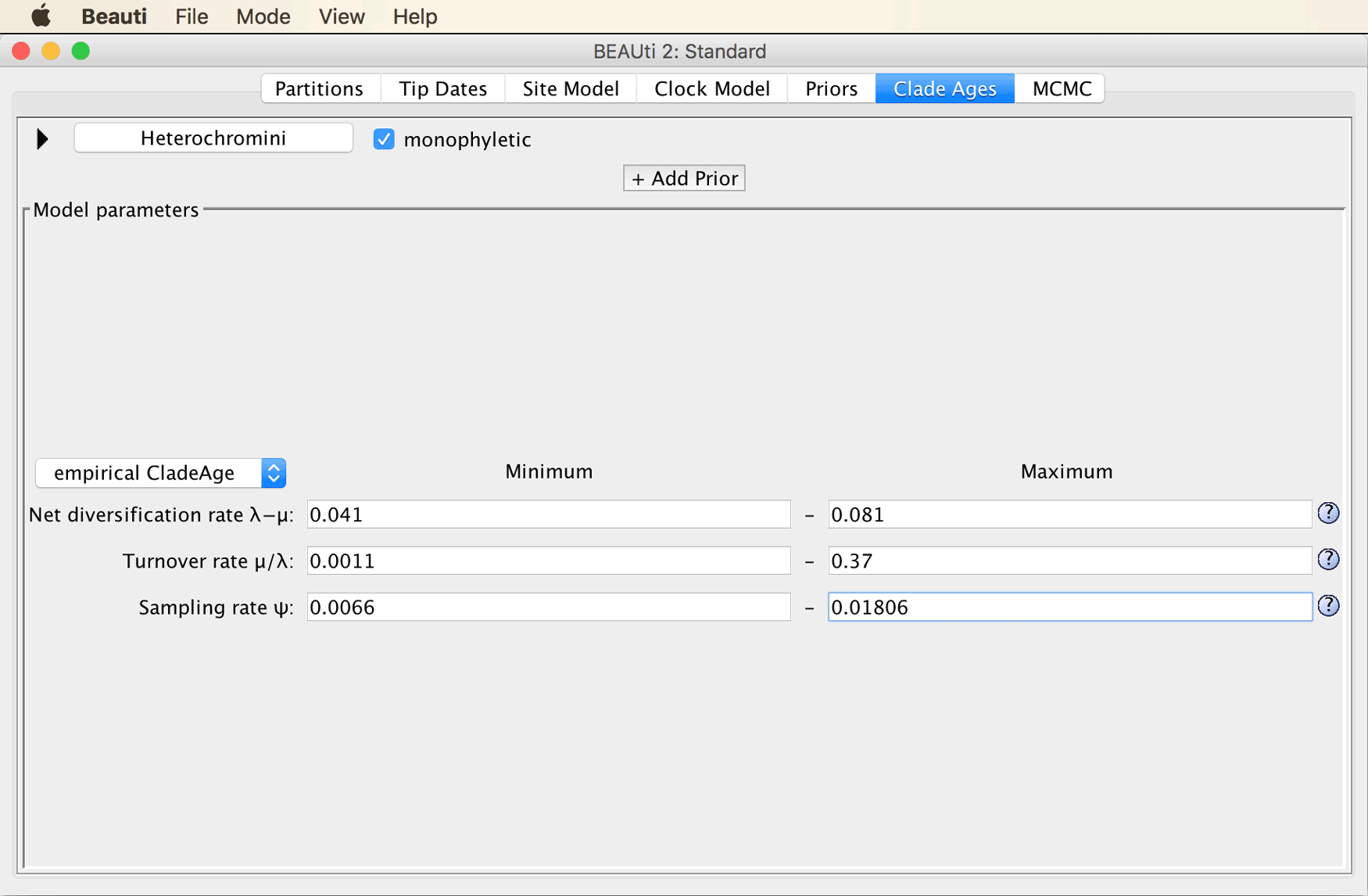
While these three rate estimates are going to apply to all fossil constraints, information specific to the fossil constraint still must be added.
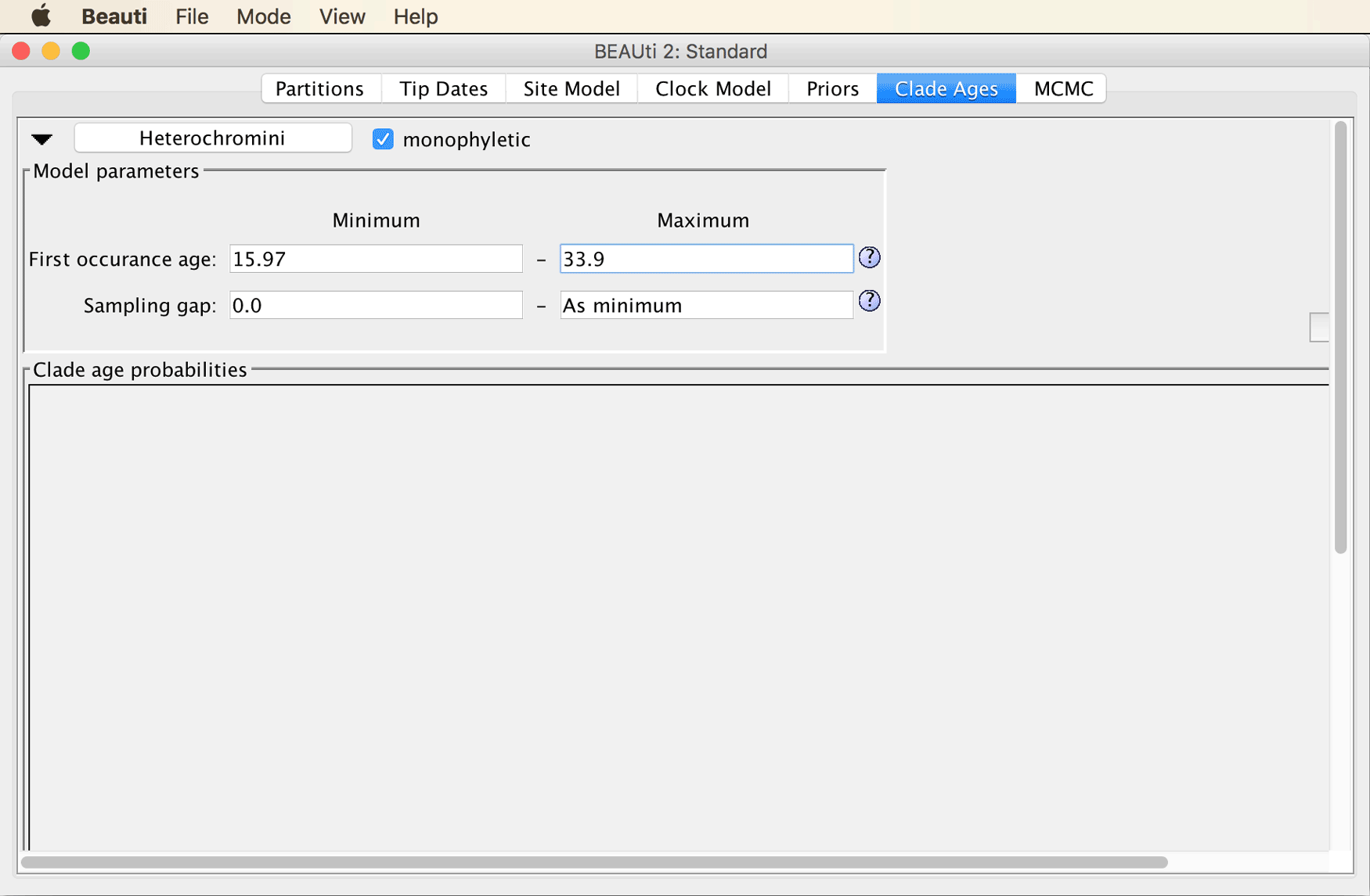
To add more information specific to the Heterochromini constraint, click on the triangle to the left of “Heterochromini”.
You’ll see four more fields in which you can specify minimum and maximum values for the “First occurrence age” (the age of the oldest fossil of the clade) and a “Sampling gap”. This sampling gap is supposed to represent a period of time right after the origin of the clade during which one might assume that either fossilization is unlikely (for example because the clade’s population might still be too small) or that fossils would not be recognized as belonging to that clade (because it might not have evolved diagnostic characters yet). We are going to ignore the possibility of a sampling gap here.
Specify the known age of the oldest fossil of Heterochromini in million of years, 15.97-33.9.
It is also possible to preview the shape of the prior densities as calculated by CladeAge based on the specified parameters.
Click on the “Preview” button below the CladeAge icon on the right (you may have to increase the window size to see it).
A plot outlining the prior densities should then appear as in the screenshot below.
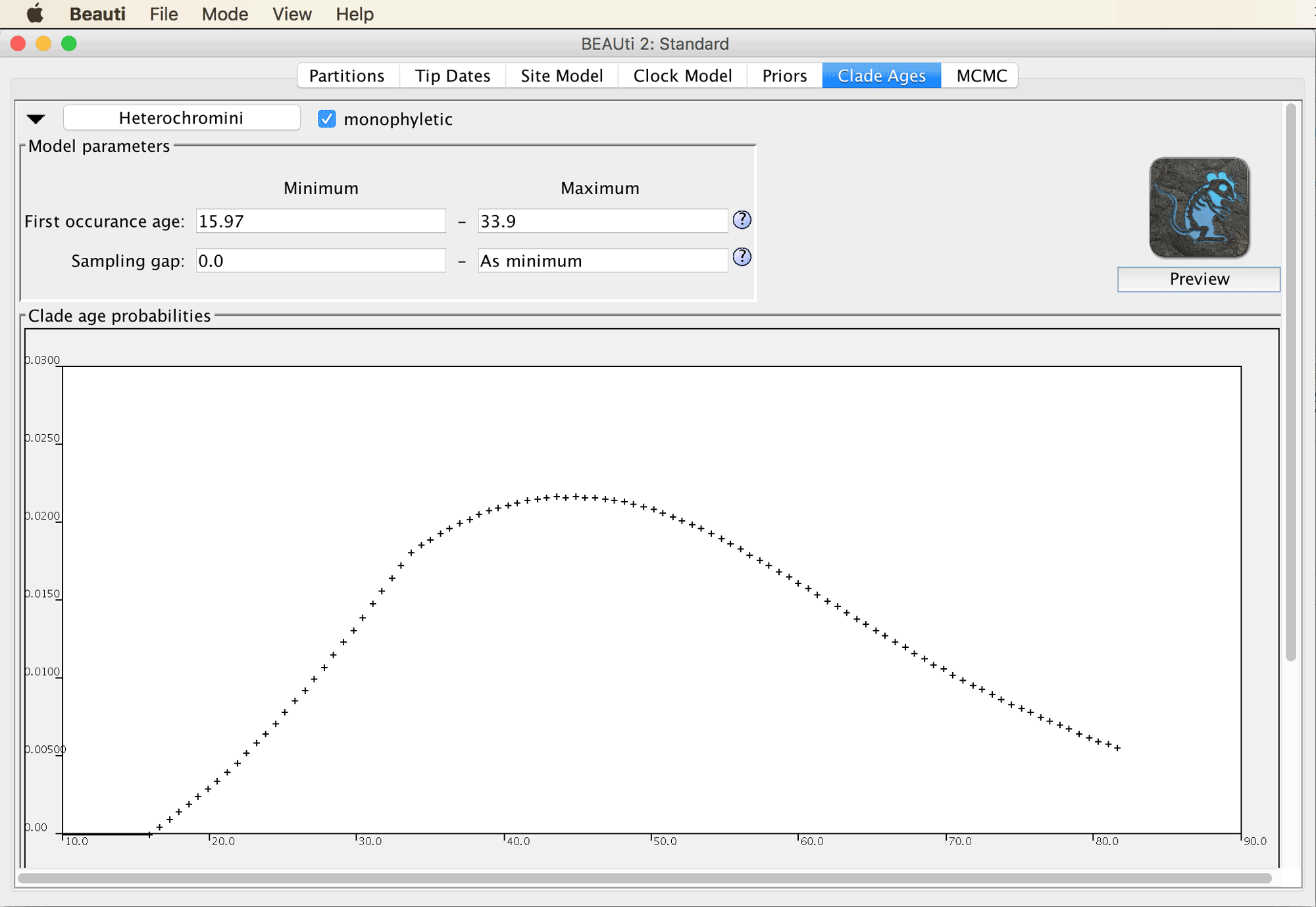
From this plot, you can see that under the assumption that all specified model parameters are correct, there’s a good probability that Heterochromini originated some time between 25 and 80 Ma. While this range is rather wide, it is based on only one fossil; we will obtain more precise estimates when we run the phylogenetic analysis with multiple fossil constraints.
Click the triangle to the left of “Heterochromini” again to close the section with details on this fossil constraint.
Add further fossil constraints for each of the clades listed below (see the Supplementary Material of Matschiner et al. (“Bayesian Phylogenetic Estimation of Clade Ages Supports Trans-Atlantic Dispersal of Cichlid Fishes,” 2017) if interested in details and references):
- “Other African cichlid tribes”
Ingroup: Oreochromis niloticus (“Oreochromis_niloticus”)
Oldest fossil species: Mahengechromis spp.
First occurrence age: 45.0-46.0 Ma - “African cichlids”
Ingroup: Heterochromis multidens (“Heterochromis_multidensA”), Oreochromis niloticus (“Oreochromis_niloticus”)
Oldest fossil species: Mahengechromis spp.
First occurrence age: 45.0-46.0 Ma - “Retroculini and Cichlini”
Ingroup: Cichla temensis (“Cichla_temensisA”)
Oldest fossil species: Palaeocichla longirostrum
First occurrence age: 5.332-23.03 Ma - “Other Neotropical cichlid tribes”
Ingroup: Heros appendictulatus (“Heros_appendictulatusA”)
Oldest fossil species: Plesioheros chauliodus
First occurrence age: 39.9-45.0 Ma - “Neotropical cichlids”
Ingroup: Cichla temensis (“Cichla_temensisA”), Heros appendictulatus (“Heros_appendictulatusA”)
Oldest fossil species: Plesioheros chauliodus
First occurrence age: 39.9-45.0 Ma - “Afro-American cichlids”
Ingroup: Cichla temensis (“Cichla_temensisA”), Heros appendictulatus (“Heros_appendictulatusA”), Heterochromis multidens (“Heterochromis_multidensA”), Oreochromis niloticus (“Oreochromis_niloticus”)
Oldest fossil species: Mahengechromis spp.
First occurrence age: 45.0-46.0 Ma - “Cichlids”
Cichla temensis (“Cichla_temensisA”), Etroplus maculatus (“Etroplus_maculatusA”), Heros appendictulatus (“Heros_appendictulatusA”), Heterochromis multidens (“Heterochromis_multidensA”), Oreochromis niloticus (“Oreochromis_niloticus”)
Oldest fossil species: Mahengechromis spp.
First occurrence age: 45.0-46.0 Ma - “Atherinomorphae”
Ingroup: Oryzias latipes (“Oryzias_latipes”)
Oldest fossil species: Rhamphexocoetus volans
First occurrence age: 49.1-49.4 Ma - “Ovalentaria”
Ingroup: Cichla temensis (“Cichla_temensisA”), Etroplus maculatus (“Etroplus_maculatusA”), Heros appendictulatus (“Heros_appendictulatusA”), Heterochromis multidens (“Heterochromis_multidensA”), Oreochromis niloticus (“Oreochromis_niloticus”), Oryzias latipes (“Oryzias_latipes”)
Oldest fossil species: Rhamphexocoetus volans
First occurrence age: 49.1-49.4 Ma - “Carangaria”
Ingroup: Trachinotus carolinus (“Trachinotus_carolinusA”)
Oldest fossil species: Trachicaranx tersus
First occurrence age: 55.8-57.23 Ma - “Anabantiformes”
Ingroup: Channa striata (“Channa_striataA”)
Oldest fossil species: Osphronemus goramy
First occurrence age: 45.5-50.7 Ma - “Anabantaria”
Ingroup: Channa striata (“Channa_striataA”), Monopterus albus (“Monopterus_albusA”)
Oldest fossil species: Osphronemus goramy
First occurrence age: 45.5-50.7 Ma - “Eupercaria”
Ingroup: Gasterosteus aculeatus (“Gasterosteus_acuC”)
Oldest fossil species: Cretatriacanthus guidottii
First occurrence age: 83.5-99.6 Ma - “Gobiaria”
Ingroup: Astrapogon tellatus (“Astrapogon_stellatusA”)
Oldest fossil species: “Gobius” gracilis
First occurrence age: 30.7-33.9 Ma - “Syngnatharia”
Ingroup: Aulostomus chinensis (“Aulostomus_chinensisA”)
Oldest fossil species: Prosolenostomus lessinii
First occurrence age: 49.1-49.4 Ma - “Pelagaria”
Ingroup: Thunnus albacares (“Thunnus_albacaresA”)
Oldest fossil species: Eutrichiurides opiensis
First occurrence age: 56.6-66.043 Ma - “Batrachoidiaria”
Ingroup: Porichthys notatus (“Porichthys_notatusA”)
Oldest fossil species: Louckaichthys novosadi
First occurrence age: 27.82-33.9 Ma - “Ophidiaria”
Ingroup: Diplacanthopoma brunnea (“Diplacanthopoma_brunneaA”)
Oldest fossil species: Eolamprogrammus senectus
First occurrence age: 55.8-57.23 Ma - “Percomorphaceae”
Ingroup: Astrapogon tellatus (“Astrapogon_stellatusA”), Aulostomus chinensis (“Aulostomus_chinensisA”), Channa striata (“Channa_striataA”), Cichla temensis (“Cichla_temensisA”), Diplacanthopoma brunnea (“Diplacanthopoma_brunneaA”), Etroplus maculatus (“Etroplus_maculatusA”), Gasterosteus aculeatus (“Gasterosteus_acuC”), Heros appendictulatus (“Heros_appendictulatusA”), Heterochromis multidens (“Heterochromis_multidensA”), Monopterus albus (“Monopterus_albusA”), Oreochromis niloticus (“Oreochromis_niloticus”), Oryzias latipes (“Oryzias_latipes”), Porichthys notatus (“Porichthys_notatusA”), Thunnus albacares (“Thunnus_albacaresA”), Trachinotus carolinus (“Trachinotus_carolinusA”)
Oldest fossil species: Cretatriacanthus guidottii
First occurrence age: 83.5-99.6 Ma - “Holocentrimorphaceae”
Ingroup: Sargocentron cornutum (Sargocentron_cornutumA)
Oldest fossil species: Caproberyx pharsus
First occurrence age: 97.8-99.1 Ma - “Acanthopterygii”
Ingroup: Astrapogon tellatus (“Astrapogon_stellatusA”), Aulostomus chinensis (“Aulostomus_chinensisA”), Channa striata (“Channa_striataA”), Cichla temensis (“Cichla_temensisA”), Diplacanthopoma brunnea (“Diplacanthopoma_brunneaA”), Etroplus maculatus (“Etroplus_maculatusA”), Gasterosteus aculeatus (“Gasterosteus_acuC”), Heros appendictulatus (“Heros_appendictulatusA”), Heterochromis multidens (“Heterochromis_multidensA”), Monocentris japonica (“Monocentris_japonicaA”), Monopterus albus (“Monopterus_albusA”), Oreochromis niloticus (“Oreochromis_niloticus”), Oryzias latipes (“Oryzias_latipes”), Porichthys notatus (“Porichthys_notatusA”), Rondeletia loricata (“Rondeletia_loricataA”), Thunnus albacares (“Thunnus_albacaresA”), Trachinotus carolinus (“Trachinotus_carolinusA”), Sargocentron cornutum (Sargocentron_cornutumA)
Oldest fossil species: Caproberyx pharsus
First occurrence age: 97.8-99.1 Ma - “Polymixiipterygii”
Ingroup: Polymixia japonica (“Polymixia_japonicaA”)
Oldest fossil species: Homonotichthys rotundus
First occurrence age: 93.5-96.0 Ma - “Percopsaria”
Ingroup: Percopsis omiscomaycus (“Percopsis_omiscomaycusA”)
Oldest fossil species: Mcconichthys longipinnis
First occurrence age: 61.1-66.043 Ma - “Zeiariae”
Ingroup: Zenopsis conchifera (“Zenopsis_conchiferaB”)
Oldest fossil species: Cretazeus rinaldii
First occurrence age: 69.2-76.4 Ma - “Gadiformes”
Ingroup: Gadus morhua (“Gadus_morhua”)
Oldest fossil species: Protacodus sp.
First occurrence age: 59.7-62.8 Ma - “Paracanthopterygii”
Ingroup: Gadus morhua (“Gadus_morhua”), Percopsis omiscomaycus (“Percopsis_omiscomaycusA”), Stylephorus chordatus (“Stylephorus_chordatusB”), Zenopsis conchifera (“Zenopsis_conchiferaB”)
Oldest fossil species: Cretazeus rinaldii
First occurrence age: 69.2-76.4 Ma
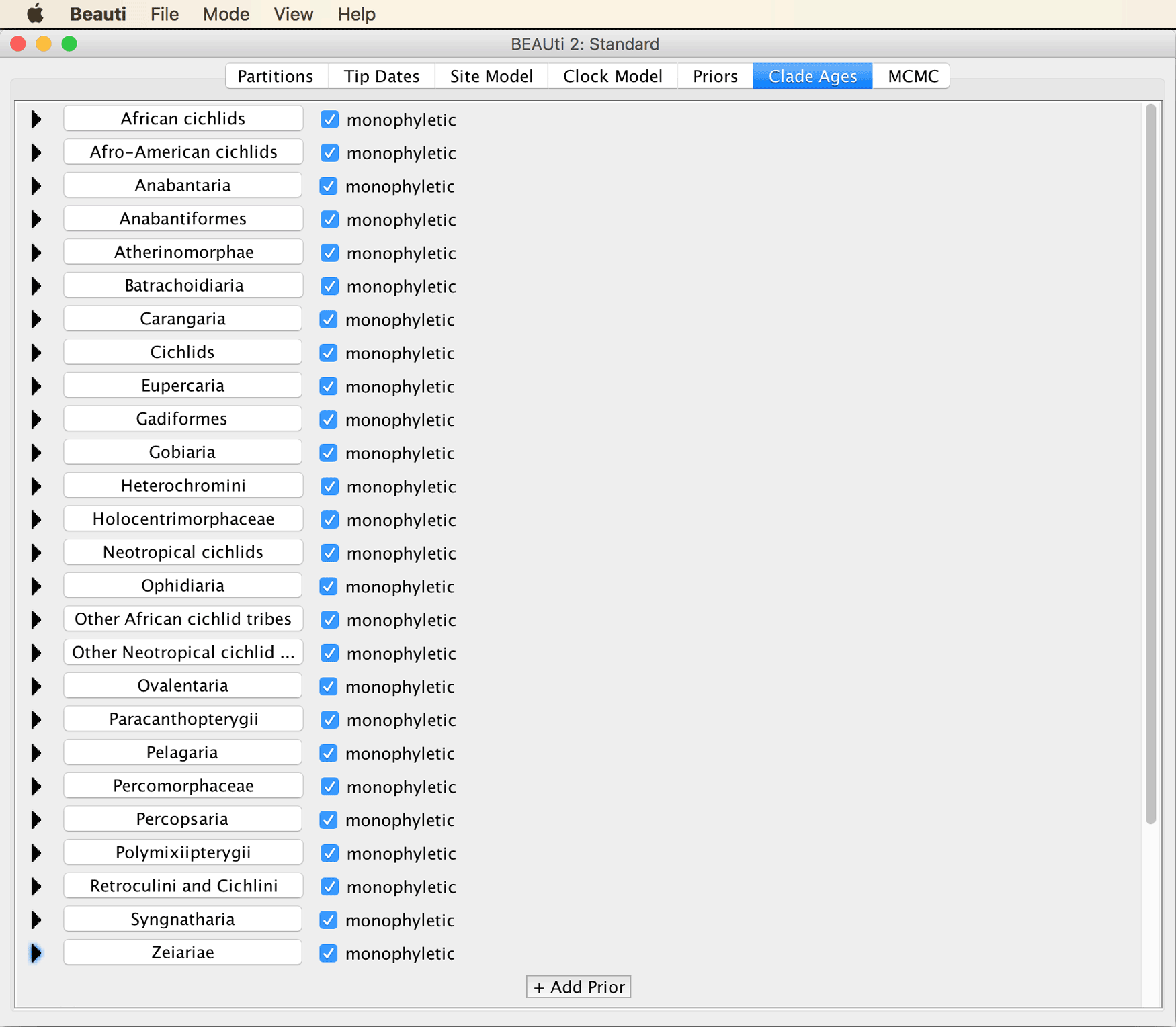
Once all these constraints are added, the BEAUti window should look as shown below.
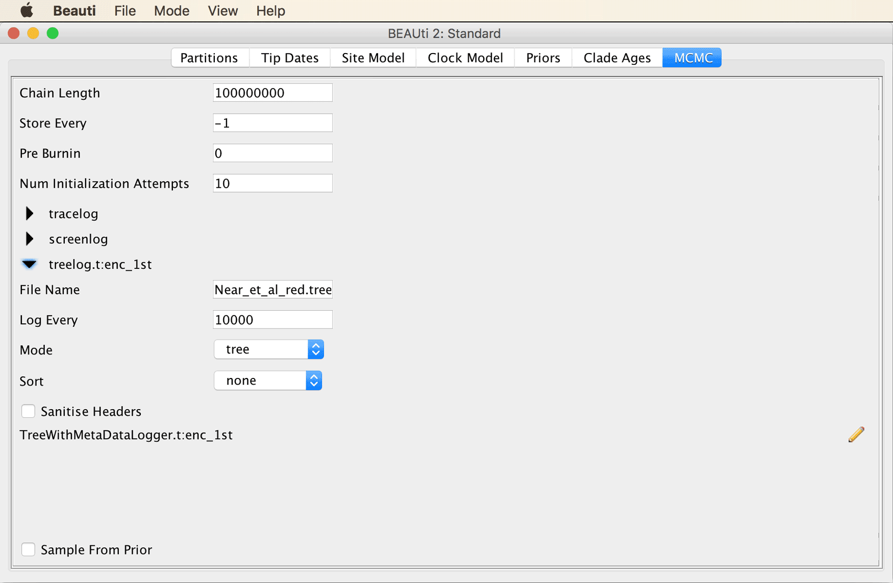
Move on to the “MCMC” tab. Specify an MCMC chain length of 100 million iterations, name the log file
Near_et_al_red.logand the tree fileNear_et_al_red.trees, and use a log frequency of 10,000 for both of these output files.
The BEAUti window should then look as in the next screenshot.
Save the analysis settings to a new file named
Near_et_al_red.xmlby clicking “Save As” in BEAUti’s “File” menu.
Running the BEAST2 analysis
Open BEAST2, load file Near_et_al_red.xml, and try running the MCMC analysis.
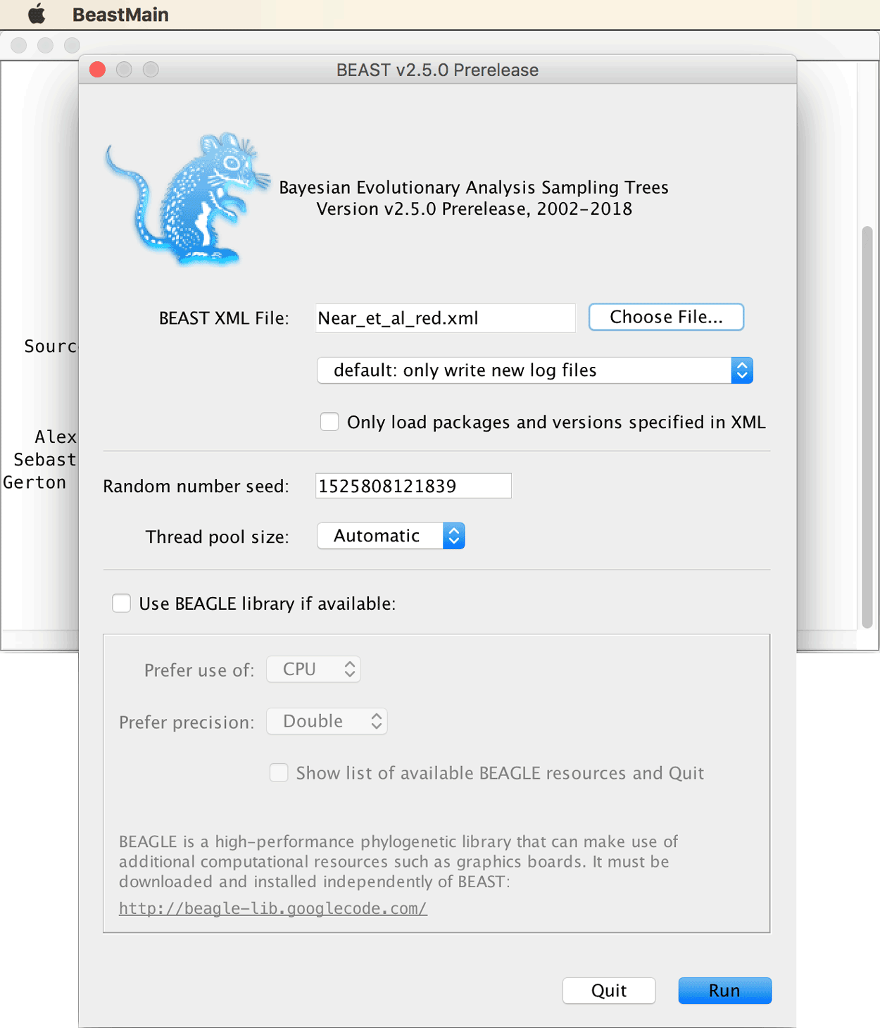
Most likely, the MCMC analysis is going to crash right at the start with an error message as shown below.
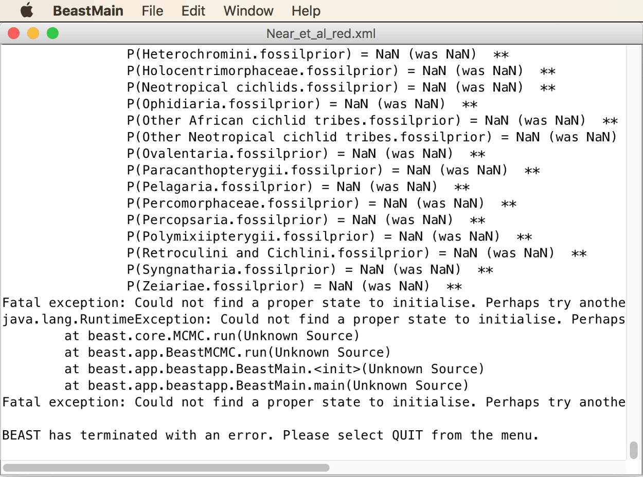
This is a common problem when several fossil constraints are specified: According to the error message, BEAST2 could not find a proper state to initialize. This means that even after several attempts, no starting state of the MCMC chain could be found that had a non-zero probability. Most often, the issue is that the tree that BEAST2 randomly generates to start the chain is in conflict with one or more fossil constraints. The way to fix this issue is to specify a starting tree that is in agreement with the specified fossil constraints. In particular, because all fossil constraints impose hard minimum ages on the origin of the respective clades, these clades must at least be as old as the minimum age in the starting tree. In case of doubt, it is usually safer to make the starting tree too old rather than too young, since the course of the MCMC chain should, at least after the burnin, not be influenced by the starting state anymore anyway. Some helpful advice on how to specify starting trees is provided on the BEAST2 webpage. With trees of hundreds of taxa, generating a suitable starting tree can be a tricky task in itself, but with the small number of 24 species used here, writing a starting tree by hand is feasible.
Copy and paste the below starting tree string into a new FigTree window.
((((((((((((((Oreochromis_niloticus:50,Heterochromis_multidensA:50):10,(Cichla_temensisA:50,Heros_appendictulatusA:50):10):10,Etroplus_maculatusA:70):30,Oryzias_latipes:100):10,(Trachinotus_carolinusA:70,(Channa_striataA:60,Monopterus_albusA:60):10):40):10,Gasterosteus_acuC:120):10,Astrapogon_stellatusA:130):10,(Aulostomus_chinensisA:80,Thunnus_albacaresA:80):60):10,Porichthys_notatusA:150):10,Diplacanthopoma_brunneaA:160):10,Sargocentron_cornutumA:170):10,(Rondeletia_loricataA:100,Monocentris_japonicaA:100):80):10,Polymixia_japonicaA:190):10,((((Gadus_morhua:70,Stylephorus_chordatusB:70):10,Zenopsis_conchiferaB:80):10,Percopsis_omiscomaycusA:90):10,Regalecus_Glesne:100):100)
Then, set a tick next to “Node Labels” to display node ages. As you’ll see, I just arbitrarily specified for most branches a length of 10 million years, and I made sure that particularly the more recent divergence events agree with the respective fossil constraints (e.g. by placing the divergence of Oreochromis niloticus and Heterochromis multidens at 50 Ma because the origin of the clade “Other African cichlid tribes”, represented by Oreochromis niloticus is constrained to be at least 45 million years old).
There are two ways to specify starting trees for BEAST2 analyses; either again using BEAUti or by editing the XML file in a text editor.
To do this with BEAUti, click on the “View” menu and select “Show Starting tree panel”, as shown in the next screenshot.
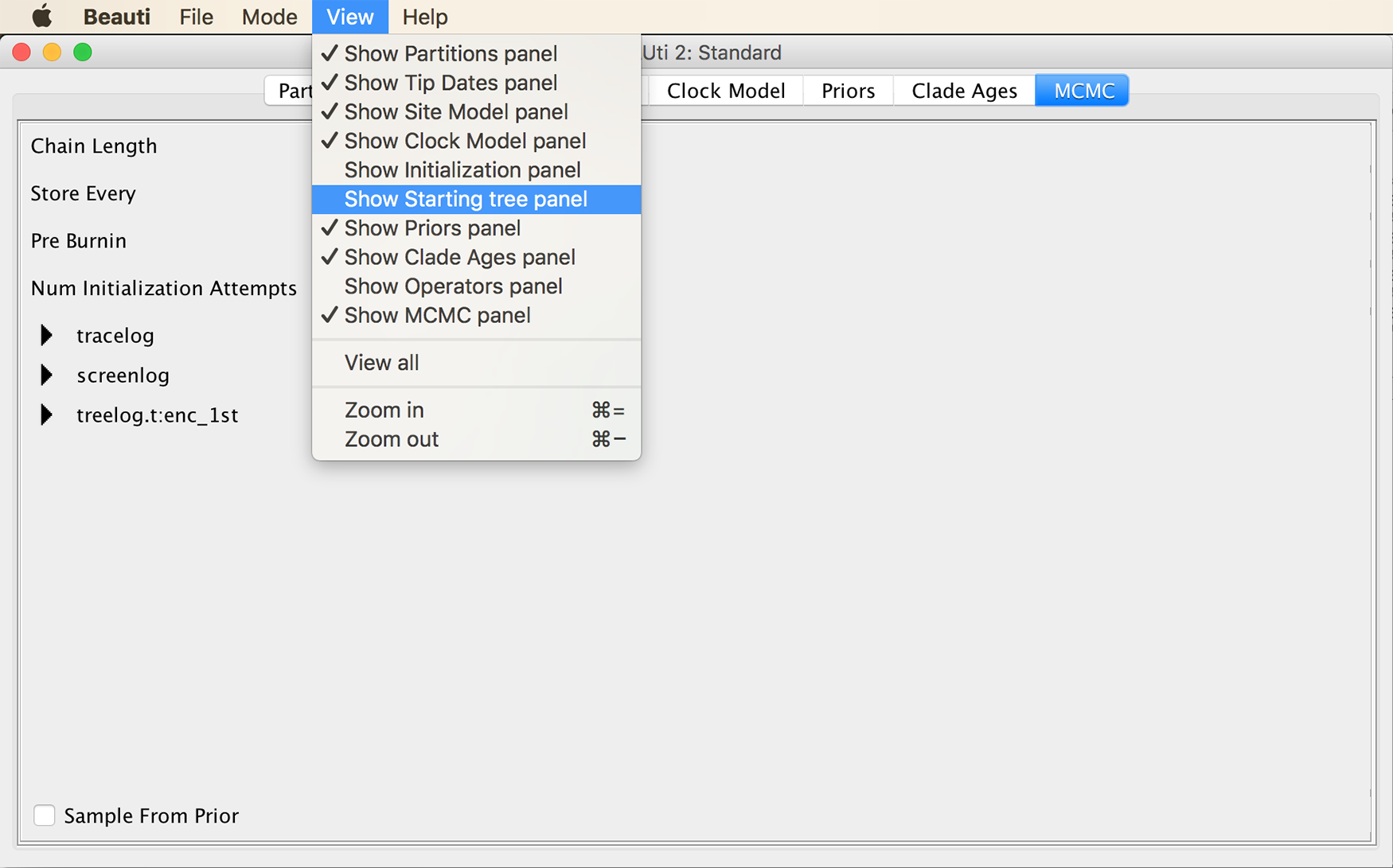
The starting tree panel should appear, as in the screenshot below.
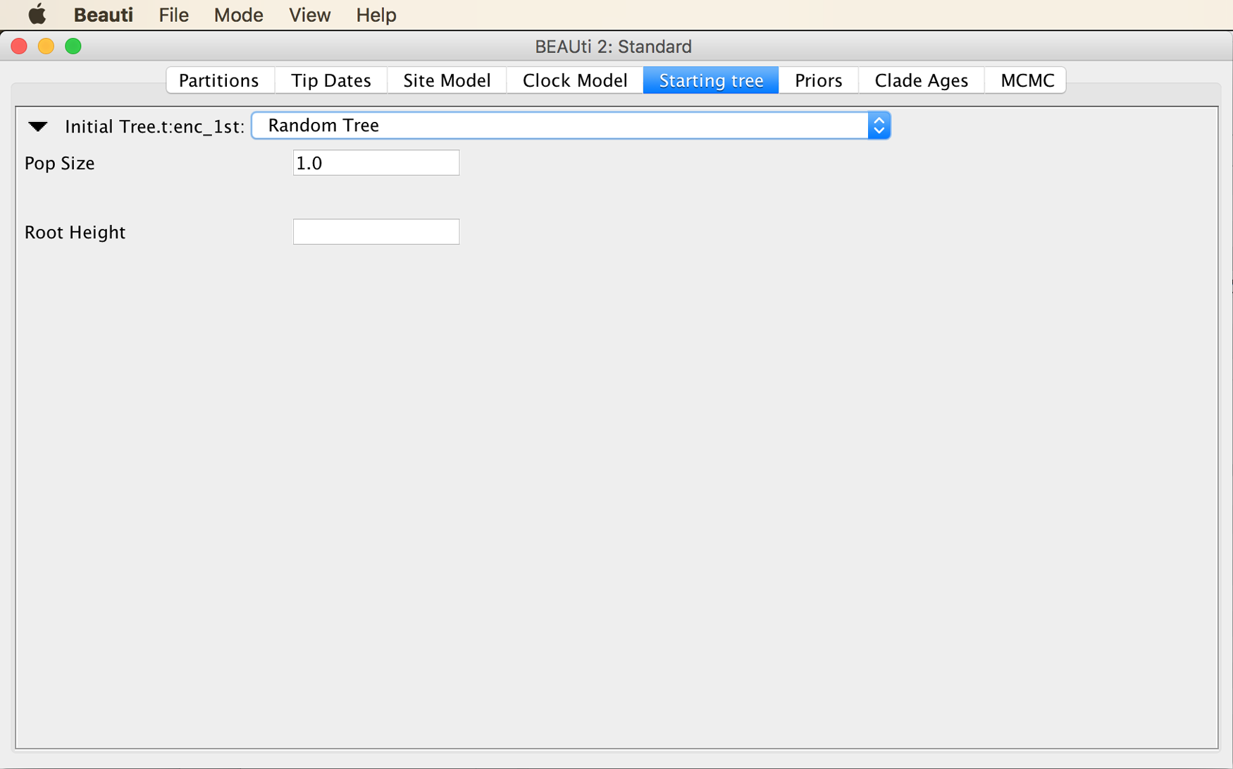
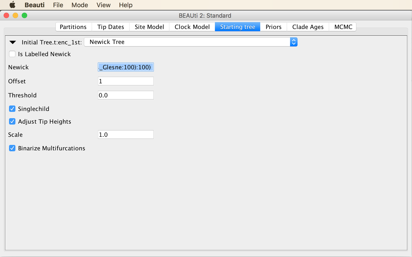
From the menu at the top of the panel, choose “Newick Tree”, as shown in the next screenshot.
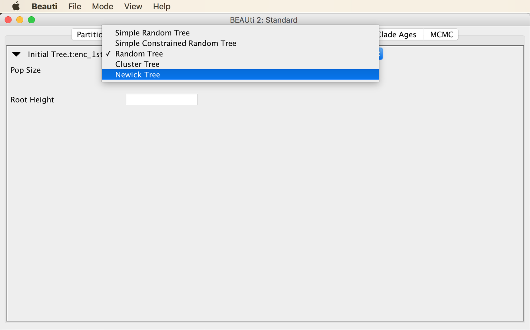
Then, copy the starting tree string into the input field next to “Newick”, as shown below.
Save the XML file again with “Save” in the “File” menu, open it again in BEAST2, and try running the analysis again. This time, the MCMC should begin to run.
If for some reason adding the starting tree in BEAUti should not work, this can alternatively be done in a text editor, as described below (if you did add it in BEAUti, you may skip the next three steps):
Open file
Near_et_al_red.xmlin a text editor and find the block shown below on lines 337-341.
		<init id="RandomTree.t:enc_1st" spec="beast.evolution.tree.RandomTree" estimate="false" initial="@Tree.t:enc_1st" taxa="@enc_1st">
			<populationModel id="ConstantPopulation0.t:enc_1st" spec="ConstantPopulation">
				<parameter id="randomPopSize.t:enc_1st" name="popSize">1.0</parameter>
			</populationModel>
		</init>
Replace the above block with the code below, which contains the starting tree string.
		<init spec="beast.util.TreeParser" id="NewickTree.t:enc_1st"
			initial="@Tree.t:enc_1st"
			IsLabelledNewick="true"
			taxa="@enc_1st"
			newick="((((((((((((((Oreochromis_niloticus:50,Heterochromis_multidensA:50):10,(Cichla_temensisA:50,Heros_appendictulatusA:50):10):10,Etroplus_maculatusA:70):30,Oryzias_latipes:100):10,(Trachinotus_carolinusA:70,(Channa_striataA:60,Monopterus_albusA:60):10):40):10,Gasterosteus_acuC:120):10,Astrapogon_stellatusA:130):10,(Aulostomus_chinensisA:80,Thunnus_albacaresA:80):60):10,Porichthys_notatusA:150):10,Diplacanthopoma_brunneaA:160):10,Sargocentron_cornutumA:170):10,(Rondeletia_loricataA:100,Monocentris_japonicaA:100):80):10,Polymixia_japonicaA:190):10,((((Gadus_morhua:70,Stylephorus_chordatusB:70):10,Zenopsis_conchiferaB:80):10,Percopsis_omiscomaycusA:90):10,Regalecus_Glesne:100):100)">
		</init>
Save the file after adding the tree string, open it again in BEAST2, and launch the analysis.
Depending on the speed of your computer, this analysis will take half a day or longer. You could cancel the BEAST2 analysis after some time if you don’t want to wait for it to finish, and you could instead continue the rest of tutorial with the prepared results that you’ll find in files Near_et_al_red.log and Near_et_al_red.trees (see links to these files in the menu to the left).
Inspecting the analysis results
We are now going to use the program Tracer to assess stationarity of the MCMC produced by the analyses with CladeAge.
Open the analysis log file
Near_et_al_red.login Tracer.
The Tracer window should then look as shown in the next screenshot.
Quickly browse through the long list of traces in the bottom left part of the window to see if any have particularly low ESS values.
We’ll ignore those parameters of the bModelTest model named “hasEqualFreqs…”. Besides these, the lowest ESS values are probably around 80, indicating that the chain is approaching stationarity, but that it should be run for more iterations for a complete and publishable analysis. Nevertheless, the degree of stationarity appears to be sufficient for our interpretation here.
With “posterior” selected in the list of parameters, click on “Trace” in the top right of the window.
You should see that after a steep increase at the very beginning of the MCMC, the posterior has remained more or less stationary after state 1E7 (10 million).
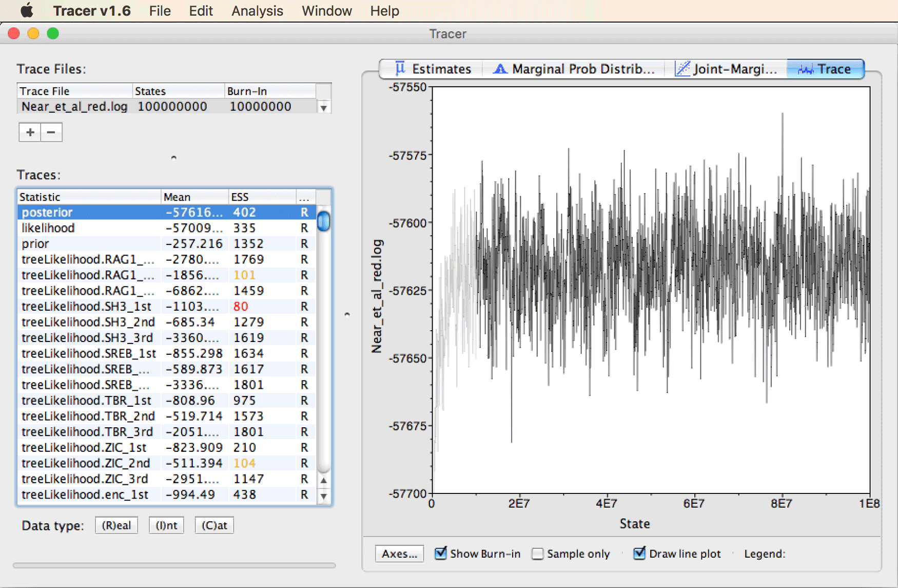
This suggest that considering the first 10% of the chain as “burn-in” is appropriate for this analysis.
To see a better example of a “hairy caterpillar” trace pattern indicating good stationarity, click on “prior” in the list of traces.
You should see a trace as shown below.
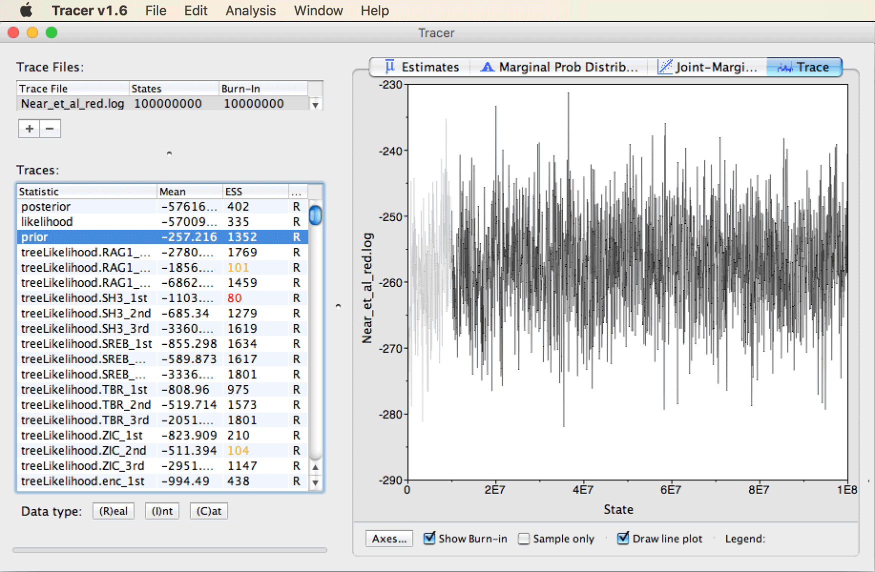
Note that in principle all traces should look similar to this pattern, with ESS values greater than 200, once the chain is fully stationary.
Select the “TreeHeight” trace indicating the root age in the list on the left.
Question 1: What is the mean estimate and its confidence interval for the age of the first split in the phylogeny? (see answer)
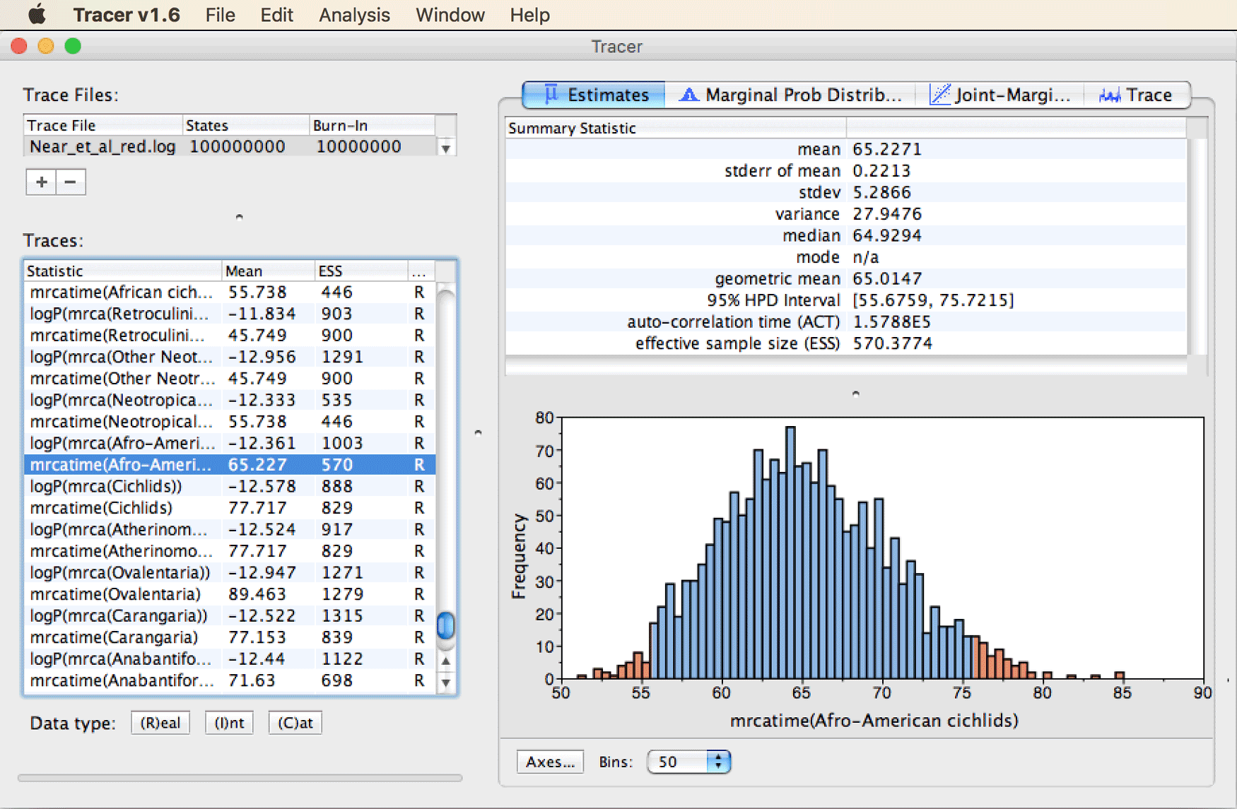
Next, find the estimated divergence time between African and Neotropical cichlid fishes. To do so, scroll to the bottom of the traces list and select “mrcatime(Afro-American cichlids)”.
You’ll see that this divergence event was estimated around 65 Ma, with a range of uncertainty between around 55 Ma and 75 Ma, as shown in the next screenshot.
Finally, select the speciation-rate parameter named “BDBirthRate” from the traces list to see the summary statistics for this parameter.
These should look similar to those shown in the screenshot below.
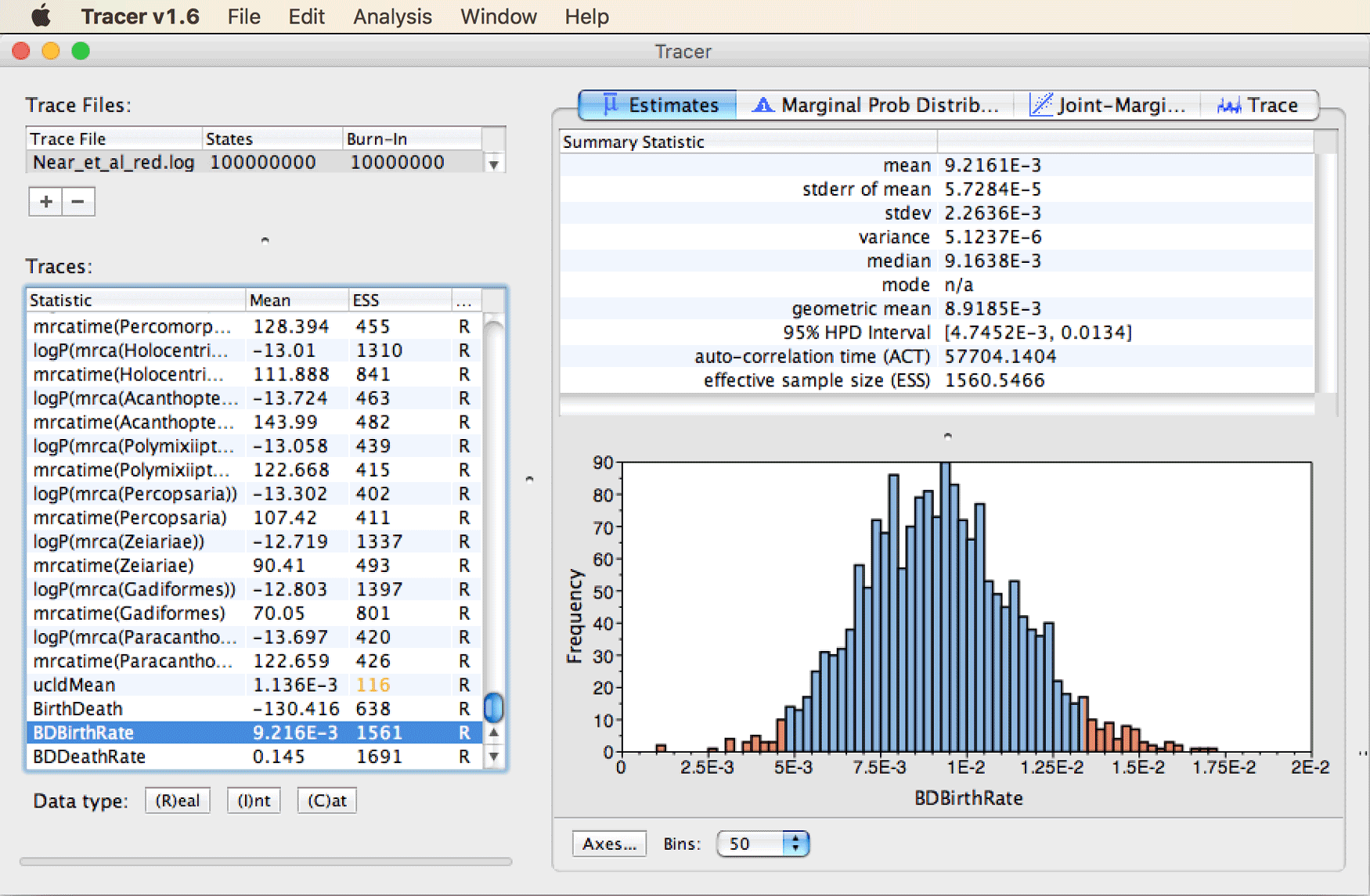
Question 2: How does this speciation-rate estimate compare to the estimate for net diversification that we used to define prior densities for CladeAge calibrations? (see answer)
Summarizing the posterior tree distribution
While analysis with Tracer has been sufficient to inspect the run stationarity and parameter estimates, we might still want to inspect and visualize the inferred tree itself. One useful method to visualize the posterior tree distribution is Densitree (Bouckaert & Heled, 2014); this software is distributed together with BEAST2. Alternatively, a single summary tree can be generated with TreeAnnotator as described below.
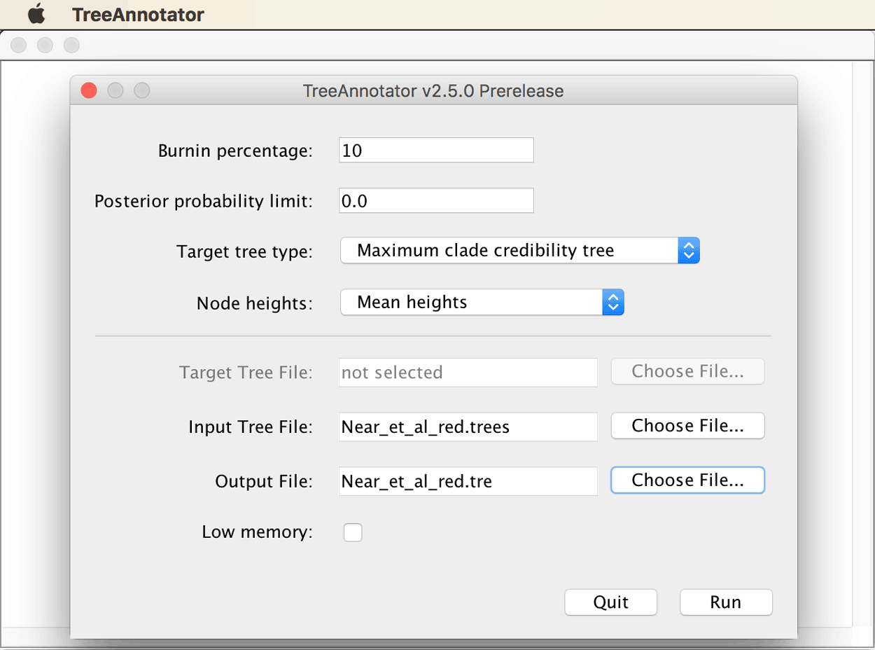
Open TreeAnnotator. Set the burn-in percentage to 10% (recall that this was determined to be appropriate based on the MCMC trace for the posterior). As the target tree type, choose “Maximum clade credibility tree” from the drop-down menu, and select “Mean heights” as node heights. Select the
Near_et_al_red.treesfile written by BEAST2 as input tree file, and name the output fileNear_et_al_red.tre.
The TreeAnnotator window should then look as shown below.
After clicking “OK”, TreeAnnotator will write the maximum-clade-credibility tree to file Near_et_al_red.tre. This tree can then be visualized with FigTree.
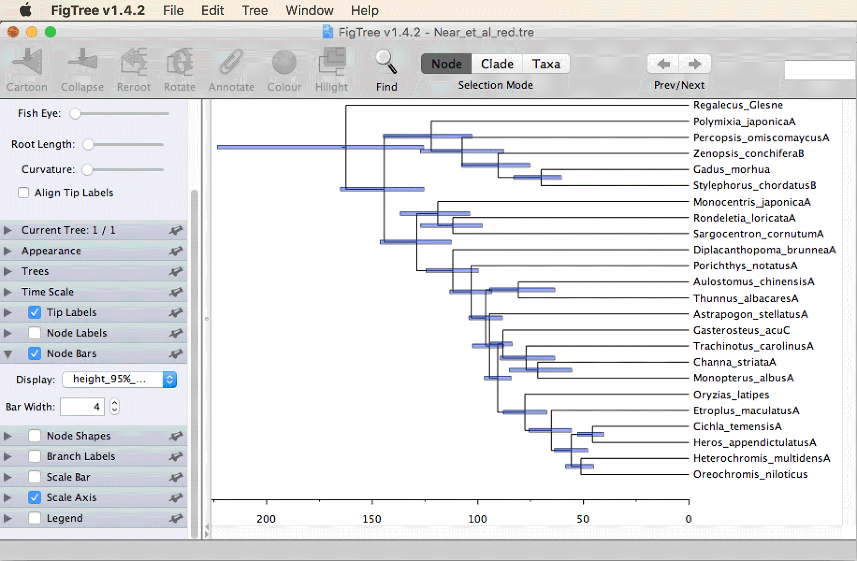
Open file
Near_et_al_red.trein FigTree. To add a time scale, set a tick next to “Scale Axis” in the menu on the left, then click the triangle next to it. Remove the tick next to “Show grid” and set a tick next to “Reverse axis”. Then, set a tick next to “Node bars”, click the triangle to open this panel, and select “height_95%_HPD” from the drop-down menu to illustrate the uncertainty in divergence-time estimates.
The tree should then be shown as in the screenshot below.
Answers to questions
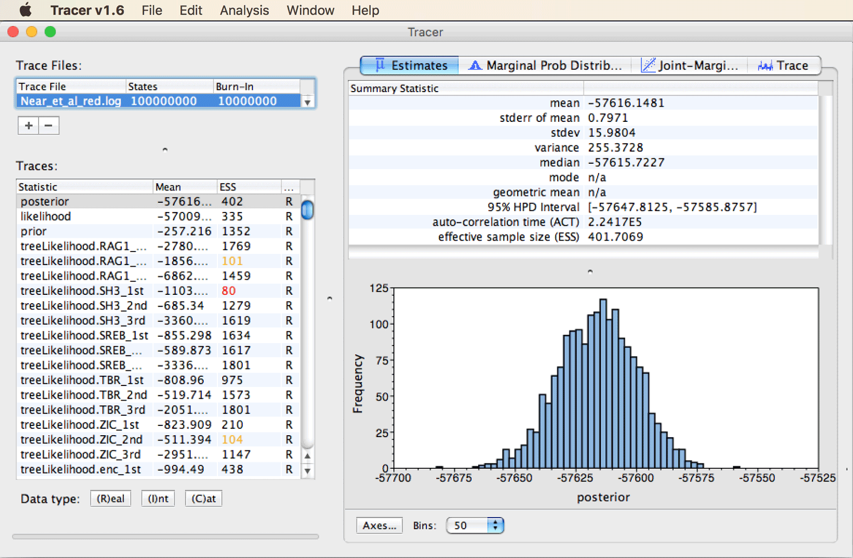
- Question 1: When you select “TreeHeight” in the list on the left and click on the tab for “Estimates” in the top right, you’ll see the following information:
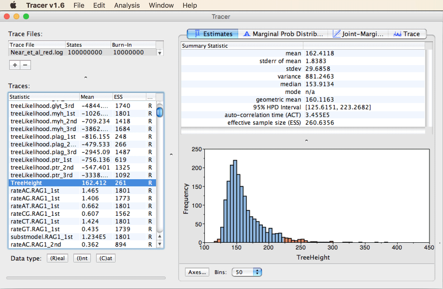
Figure A1: Analyzing results with Tracer.
</figure>As specified in the summary statistics on the top right part of the window, the mean estimate for the age of the first split should be around 160 Ma. The confidence interval is reported as the “95% HPD interval”, the highest-posterior-density interval containing 95% of the posterior distribution. In other words, this is the shortest interval within which 95% of the samples taken by the MCMC can be found. In this case, it is relatively wide, ranging from around 125 Ma to about 225 Ma.
- Question 2: The estimated speciation rate is far lower than the values that we assumed when we specified prior densities for clade ages with CladeAge. Recall that we had used the estimates for the net diversification rate from Santini et al. (“Did Genome Duplication Drive the Origin of Teleosts? A Comparative Study of Diversification in Ray-Finned Fishes,” 2009), which were 0.041-0.081 (per millon year). Thus, the estimated speciation of around 0.0009 is almost an order of magnitude lower than the values that we had assumed for the net diversification rate. This is remarkable because the speciation rate should always be higher than the net diversification rate, given that the latter is defined as the difference between the speciation and extinction rates. The explanation for this difference is that BEAST2 estimated the speciation rate under the assumption that the species that we included in the phylogeny are in fact all the extant species that descended from the root of the phylogeny. This means that BEAST2 assumed that no spiny-rayed fish species besides those 24 included in the phylogeny exist. On the other hand the estimates for the net diversification rate obtained by Santini et al. (“Did Genome Duplication Drive the Origin of Teleosts? A Comparative Study of Diversification in Ray-Finned Fishes,” 2009) accounted for the fact that only a subset of the living species were included in their phylogeny. Thus, the speciation-rate estimate resulting from our analysis is most certainly a severe underestimate. This bias, however, should not lead to strong bias in the timeline inferred in the analysis with CladeAge, because it did not influence the prior densities placed on clade ages.
Useful Links
- Rough Guide to CladeAge
- Bayesian Evolutionary Analysis with BEAST 2 (Drummond & Bouckaert, 2014)
- Ask questions at the BEAST user discussion: http://groups.google.com/group/beast-users
Relevant References
- Bouckaert, R., Heled, J., Kühnert, D., Vaughan, T., Wu, C.-H., Xie, D., Suchard, M. A., Rambaut, A., & Drummond, A. J. (2014). BEAST 2: a software platform for Bayesian evolutionary analysis. PLoS Computational Biology, 10(4), e1003537. https://doi.org/10.1371/journal.pcbi.1003537
- Near, T. J., Dornburg, A., Eytan, R. I., Keck, B. P., Smith, W. L., Kuhn, K. L., Moore, J. A., Price, S. A., Burbrink, F. T., Friedman, M., & Wainwright, P. C. (2013). Phylogeny and tempo of diversification in the superradiation of spiny-rayed fishes. Proceedings of the National Academy of Sciences USA, 110(31), 12738–12743.
- Matschiner, M., Musilová, Z., Barth, J. M. I., Starostová, Z., Salzburger, W., Steel, M., & Bouckaert, R. R. (2017). Bayesian phylogenetic estimation of clade ages supports trans-Atlantic dispersal of cichlid fishes. Systematic Biology, 66(1), 3–22.
- Betancur-R, R., Wiley, E. O., Arratia, G., Acero, A., Bailly, N., Miya, M., Lecointre, G., & Ortı́ Guillermo. (2017). Phylogenetic classification of bony fishes. BMC Evolutionary Biology, 17, 162.
- Bouckaert, R. R., & Drummond, A. J. (2017). bModelTest: Bayesian phylogenetic site model averaging and model comparison. BMC Evolutionary Biology, 17, 42.
- Lippitsch, E., & Micklich, N. (1998). Cichlid fish biodiversity in an Oligocene lake. Ital. J. Zool., 65(Suppl.), 185–188.
- Santini, F., Harmon, L. J., Carnevale, G., & Alfaro, M. E. (2009). Did genome duplication drive the origin of teleosts? A comparative study of diversification in ray-finned fishes. BMC Evolutionary Biology, 9(1), 194.
- Foote, M., & Miller, A. I. (2007). Principles of Paleontology (3rd ed.). W. H. Freeman.
- Bouckaert, R. R., & Heled, J. (2014). DensiTree 2: seeing trees through the forest. BioRxiv. https://doi.org/10.1101/012401
- Drummond, A. J., & Bouckaert, R. R. (2014). Bayesian evolutionary analysis with BEAST 2. Cambridge University Press.
Citation
If you found Taming the BEAST helpful in designing your research, please cite the following paper:
Joëlle Barido-Sottani, Veronika Bošková, Louis du Plessis, Denise Kühnert, Carsten Magnus, Venelin Mitov, Nicola F. Müller, Jūlija Pečerska, David A. Rasmussen, Chi Zhang, Alexei J. Drummond, Tracy A. Heath, Oliver G. Pybus, Timothy G. Vaughan, Tanja Stadler (2018). Taming the BEAST – A community teaching material resource for BEAST 2. Systematic Biology, 67(1), 170–-174. doi: 10.1093/sysbio/syx060